DataOps & MLOps
This documentation contains information about uploading and updating data, as well as about the lifecycle of a forecasting job sequence or an anomaly detection job sequence when solving a business problem in production. All those data-related operations and all those job-related operations don't happen independently however, but they are fundamentally interwoven. Typically, each inference (job or MLOps action) will happen only after new data has become available (dataset version or DataOps action). Similarly, each time new information shows up (DataOps action), a new inference should be made (MLOps action) to learn from this information.
Because of their tightly-coupled nature, it makes sense to have a look at DataOps and MLOps in combination with each other, and how to decide which action is appropriate for which situation. This section zooms in on the intertwined lifecycle of models and data and the different stages of this lifecycle. It explains which actions can be taken in which stage, and how these actions can be completed.
There are three major stages in the lifecycle of data and models, namely experimentation, production and reflection. It is important to realize that this is not a linear lifecycle, where each step would be completed sequentially, and then the story would be told. Rather, this is meant to be a continuous cyclical lifecycle: it starts out with experimentation, which - when successful - results in production; production then is used to gain insights and is continuously reflected on; and during this reflection it becomes clear if and when to return to experimentation. The goal of this process is to gain valuable business insights and continue to do so over time. This process ensures the right adjustments can be made at the right time to avoid outdated models, expired insights and wrong decisions.
Experimentation
Experimentation is all about getting to know the data and problem at hand, from the very first upload to confidence in model building settings. It can include more than this: in some cases, it makes sense to asses the impact of different conditions (different data) on results, and in these cases TIM can be of help too.
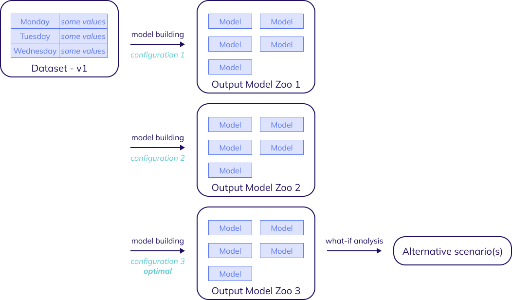
Experimentation thus encompasses everything from uploading the initial dataset, to building several models with different configurations until the optimal configuration for the use case is found, and performing what-if analysis and looking at alternative scenarios and outcomes.
Initial dataset
The first step is always to upload the initial dataset, thereby also creating the first version of the dataset. Make sure the data is in the right format, and the exploring can start.
Model building
After initializing the dataset, the model building process takes off. This is arguably the most hands-on part of the lifecycle, during which different data transformation options are tried out - such as imputation, timescaling and aggregation and filtering - and many forecasting configuration or anomaly detection (either kpi-driven or system-driven) configuration combinations are compared.
These settings can be tweaked and adjusted until the ideal match is found for the business challenge at hand, tuned to both the desired output and the nature of the problem. Depending on the use case, this will result in a configuration finely tweaked with domain expertise or one that's close to TIM's default behavior. Whatever the result is, once the user is satisfied with the results, they can move on to the production stage.
What-if analysis
Both TIM Forecast and TIM Detect offer features for what-if analysis. When a business challenge requires assessing the impact of differnt conditions (different data) could have on results - for example because that data is volatile, uncertain or can be changed at will - TIM's what-if analysis features can be of use. What-if analysis allows people to analyze different scenarios by changing input variables and observing the model outputs. It can help in recognizing the impact of individual variables on the target or KPI variable and thus make the process more efficient or reveal critical situations.
For use cases where what-if analysis is relevant, these jobs can even be taken into the production stage of the lifecycle too, so actual business decisions can be based on the insights they bring in terms of the expected range of the results.
Production
The production stage revolves around gaining insights from your data, making decisions based on these insights and adjusting where needed.
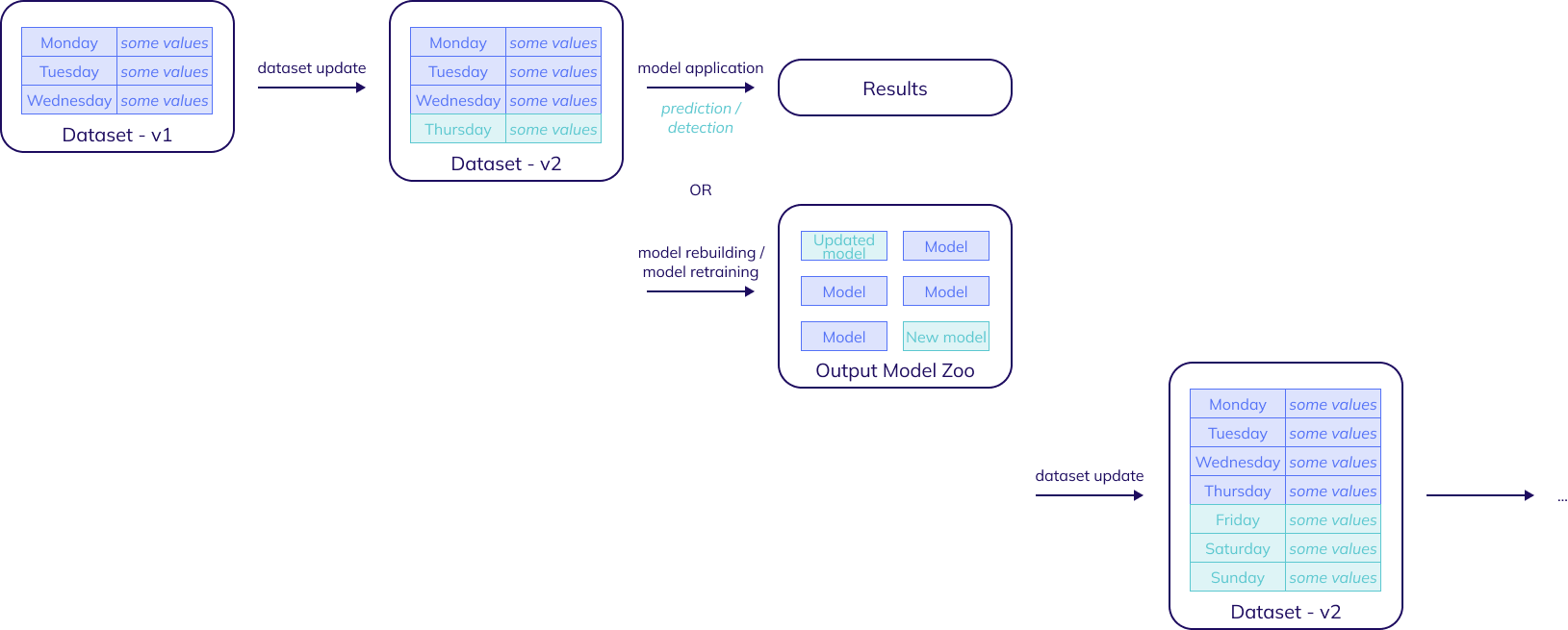
As explained before, each inference (job or MLOps action) will typically happen only after new data has become available (dataset version or DataOps action) and similarly, each time new information shows up (DataOps action), a new inference should be made (MLOps action) to learn from this information. This means that in order to move to production, dataset updates and ML jobs will alternate.
In other words, the production stage takes the form of an alternating cycle of dataset updates and model applications and model adjustments. This section looks at both of these operations in detail.
Dataset updates
In order to get the most value out of the production stage, it is important to understand when and how the dataset should be updated, meaning when and how new versions should be created.
In essence, a dataset update is a PATCH operation, meaning that only the data needs to change should be sent over. This includes additions, corrections and even removals, but the data that is already present in the previous version does not have to be resent.
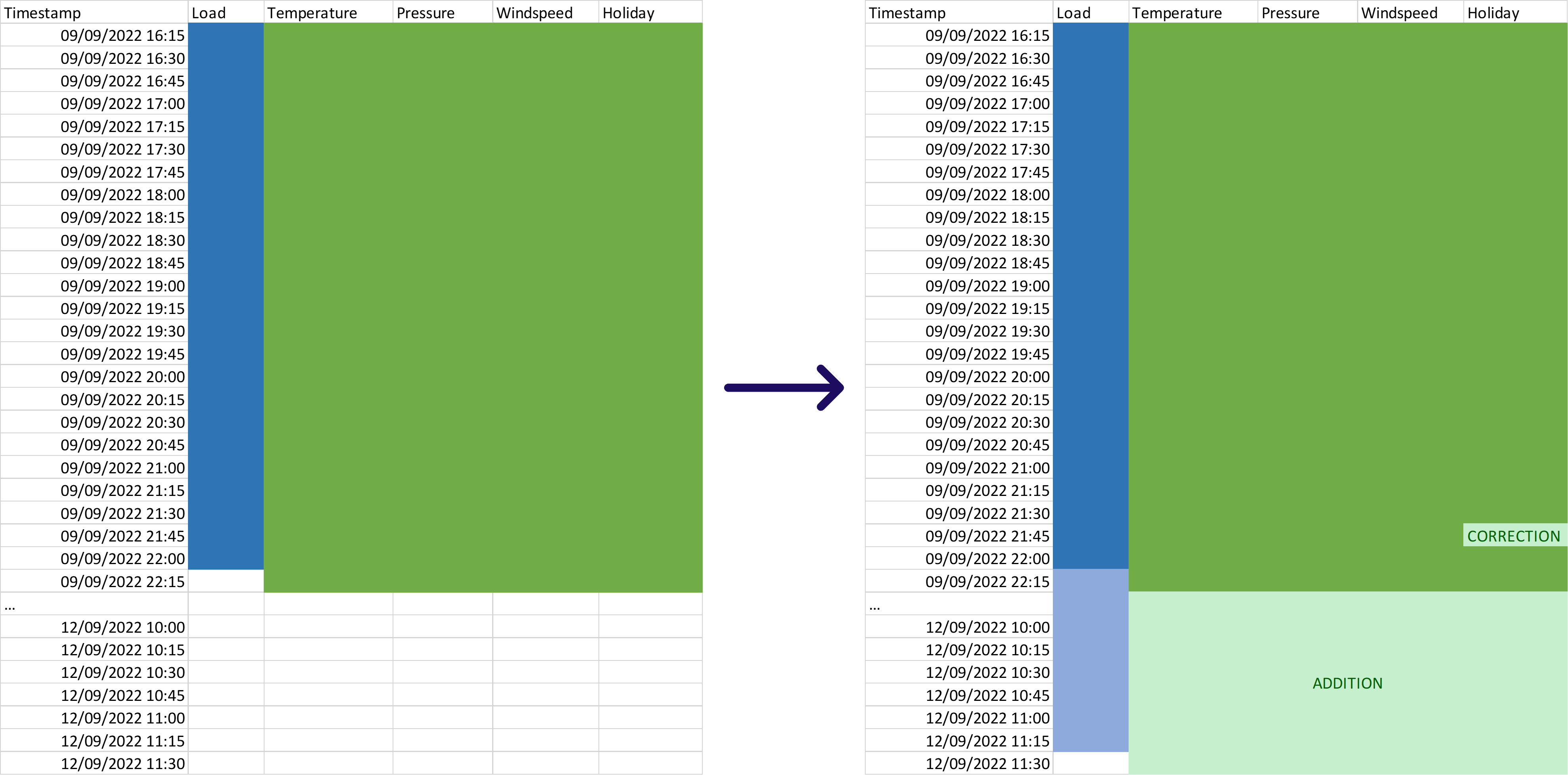
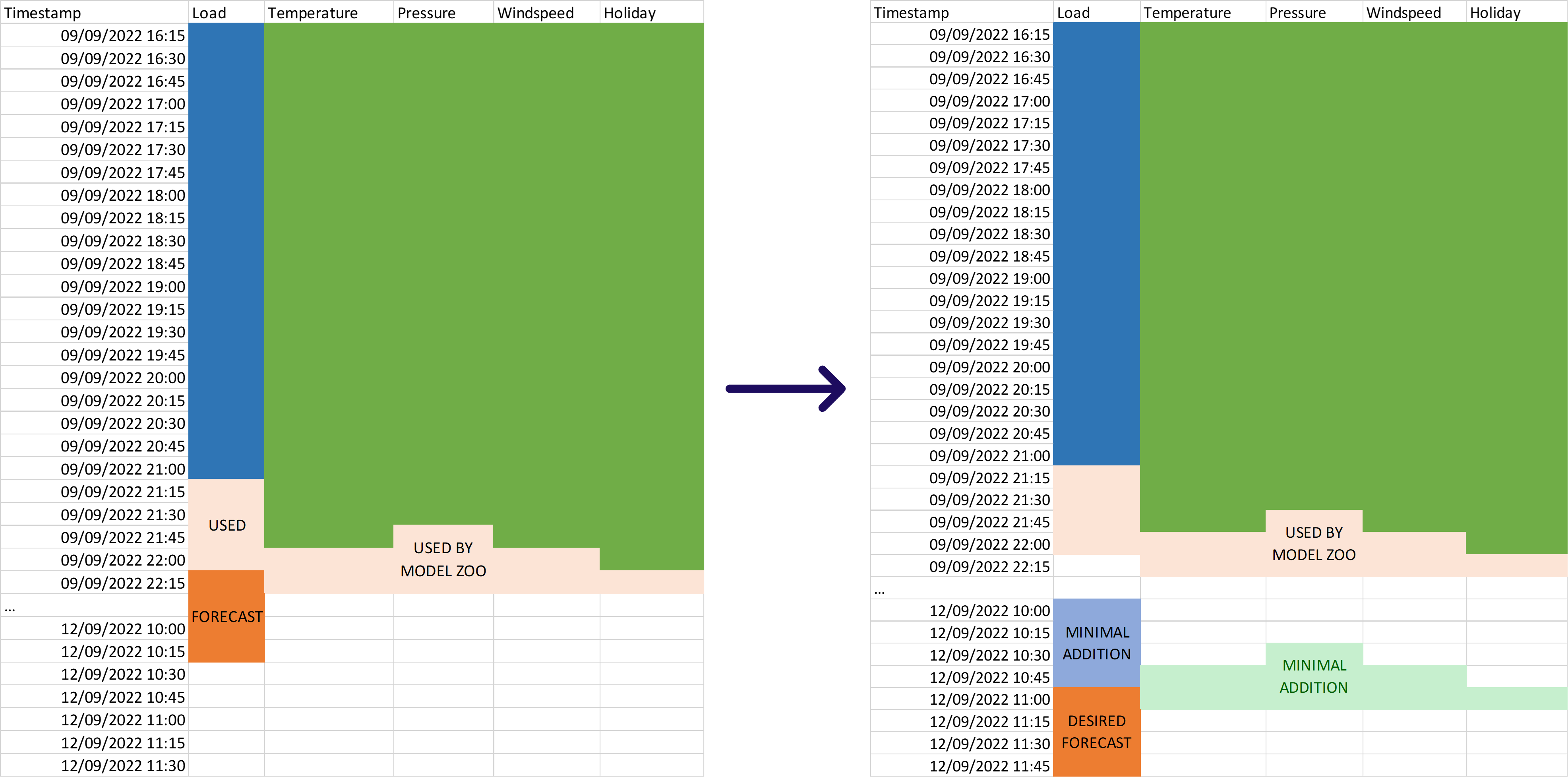
The image above shows a complete update, where the previous dataset is (corrected and) appended with the newly available data. In some cases, not all data might be available, or the user might have some other reason to prefer not doing a complete update. For such cases, it is possible to figure out what a minimal data update should look like, so that the production stage can still go on as desired. Any update between the minimal update and the complete update can be made to successfully go through the production stage.
The model building step during the experimentation stage results in an initial Model Zoo that will be used as a starting point in the production stage. Inside this Model Zoo, each model contains (among other things) its variable offsets. This information indicates how much continuous history of each predictor (or influencer) is required to be able to evaluate the model (i.e. to execute prediction jobs based on the model). The amount of observations used by the model can be used to inform the minimal amount of observations that should be included in the dataset update, as indicated in the image below.
Complete versus minimal dataset updates
Both complete dataset updates and minimal dataset updates have their advantages and disadvantages. In most cases, the best option is to opt for complete dataset updates, as the advantages outweigh the limited disadvantages. It is however up to each user if they want to compare both options and make their own informed decision. To support this, this section summarizes the advantages and disadvantes of both approaches.
A complete update ensures that the full correct data is stored in TIM DB, which also results in more data available for rebuilding (the offsets of the used data might change after rebuilding) and the possibility to perform production accuracy evaluation during the reflection stage. It does however mean all data needs to be sent over (so heavier requests) and more storage is used.
A minimal update on the other hand, means less data needs to be sent over (so lighter requests) and ensures minimal storage is used in TIM DB. However, it also means incomplete (or even incorrect/uncorrected) data might be stored, resulting in turn in minimal available data for rebuilding (so, less opportunity for improvement) and potentially hindering the the possibility for production accuracy evaluation during the reflection stage.
Model applications and model adjustments
Each time a dataset has been updated, the new information in this new version can be leveraged to gain new insights. There's two major ways to do this: by applying the model zoo built during experimentation through prediction or detection jobs, or by adjusting that model zoo through forecasting or anomaly detection rebuild jobs or even forecasting retraining jobs.
While prediction jobs, detection jobs and retraining jobs will work fine even with minimal data updates, forecasting and anomaly detection rebuild jobs can greatly benefit from complete data updates, as the new model zoo is then free to use more data then the original one did.
Reflection
The reflection stage ensures the job sequence maintains its performance. That means that it serves to inform users on when to adjust and adapt (ex.g. by taking the model adjustments track of rebuilding or retraining in the production stage, or returning to looking for the optimal configuration in the experimentation stage), so that the performance stays at least on the same level, or potentially even improves. It also allows users to gain a deeper understanding of the model zoos being used as well as the root cause behind particular (potentially strange) outputs from the jobs.
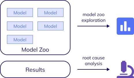
Model zoo exploration
One of the outputs of the experimentation stage is a model zoo that produces satisfying results. From that point onwards, each job should be reflected on to get all possible benefits from TIM's capabilities. This means both this original model zoo kicking of the production stage and any other model zoo resulting from forecasting or anomaly detection rebuilding or forecasting retraining actions during model adjustments can deliver additional insights and understanding through model zoo exploration.
Production accuracy evaluation
While the job sequence unfolds, circumstances, context, data... may change, and that may influence the performance. Therefore, it is important to reflect on the predictions coming out of the production stage be able to track the performance. This way, it is possible to steer and adapt with model adjustments, potentially accompanied by updated configuration settings where needed.
Production accuracy evaluation is currently only possible in TIM Forecast and effectivaly allows for evaluating the production forecasts of the jobs in the sequence after the facts, by comparing their forecasted values with the actuals that have been added to the dataset since. Therefore, when accuracy starts deteriorating, the model zoo can be altered to get back on track in terms of performance.
The results of production accuracy evaluation also serve as an indication of where to apply root cause analysis: specifically those instances where performance suddenly and strongly deteriorates can be very interesting to further investigate, leading to a deeper understanding of the data and/or business problem in focus.
Root cause analysis
In addition, each predicted value (be it a forecast or an anomaly detection) - whether it comes from one of those previous actions or from model application - can be further analyzed with root cause analysis, both in forecasting and in kpi-driven anomaly detection.