Imputation

TIM tries to parse every value to a float. If it cannot, it will consider the value to be missing. Examples of values interpreted as missing are null values, categorical (non-Boolean) valuables, NA strings and infinity markers. However, TIM offers multiple ways to impute missing data, allowing users to continue working with their data even if there are gaps in it. Additionally, TIM can handle non-imputed missing values, if the user prefers not to impute them.

Imputation is the process of replacing missing data with substituted values; different ways of imputing often indicate different ways of calculating the replacing value. Since missing values tend to make it harder to handle the data and can negatively impact model quality, it is often desired to impute them in some way so the data can afterwards be treated as if there was no missing data.

Imputation types

As mentioned above, TIM offers multiple ways to impute missing data. Currently supported imputation types include:

• LOCF or last observation carried forward: the last non-missing observation is used to replace the subsequent missing observation(s),
• linear imputation: a linear function is calculated connecting the observations on both sides of the missing observation(s) and the value(s) on this line replace(s) the missing observation(s), and
• no imputation: the value remains missing.

Maximum gap length

The maximum gap length of missing values to be imputed can be configured by the user. This is useful - among other scenarios - when dealing with regularly missing data: if for example data are missing for every weekend, the maximum imputation length can be set to cover these regular gaps (e.g. in case of hourly sampled data the maximum gap length can be set to 48).

Imputing only timestamps

TIM also supports imputing only the timestamps of the data, without imputing any actual observed values. Imputing only the timestamps of the data has no effect on any analysis TIM performs on the data afterwards (during model building and model application). When using this setting, all rows with timestamps as determined by the timescale will be returned. This means even 'empty' rows, for which all variable observations are missing, will be returned. When not using this setting, only rows with at least one non-missing variable (one observation present) will be returned.

This feature is especially useful when visualizing the data returned by TIM, as it allows the user to more easily meet the requirements and expectations of their visualization library of choice.

Special cases of missing data

Regularly missing data

Regularly missing data is data in which the missing values or gaps themselves follow a regular pattern. An example of such a use case is trading that happens only on weekdays, resulting in regular gaps covering the weekend days. Another example can be found in sales, where products are sold only during a shops opening hours, and any other hours don't have observations. Yet another example is found in the energy industry, where solar pannels don't produce electricity during nighttime and sensors may thus very well be switched off from measuring.

If desired, such data can be imputed by selecting the imputation type of choice and setting the maximum gap length to cover the regularly missing period.

Example

Have a look at the following hourly-sampled foreign exchange dataset, which clearly shows regular gaps.

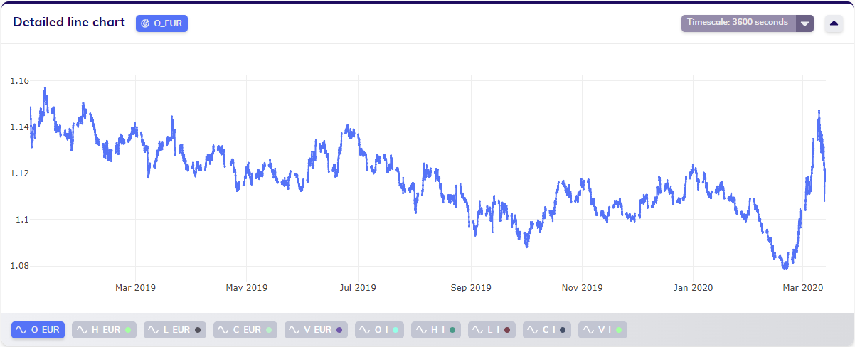
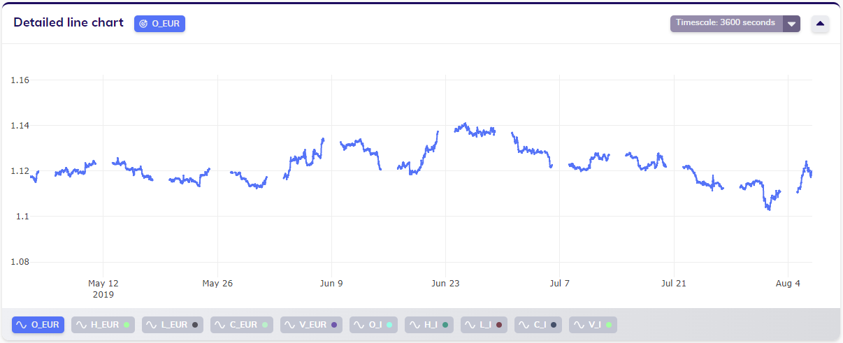
Zooming in on this data makes it even clearer that only weekdays contain data, whereas weekends do not. This makes sense, given the nature of the use case: the foreign exchange market is not available for trading on weekends.

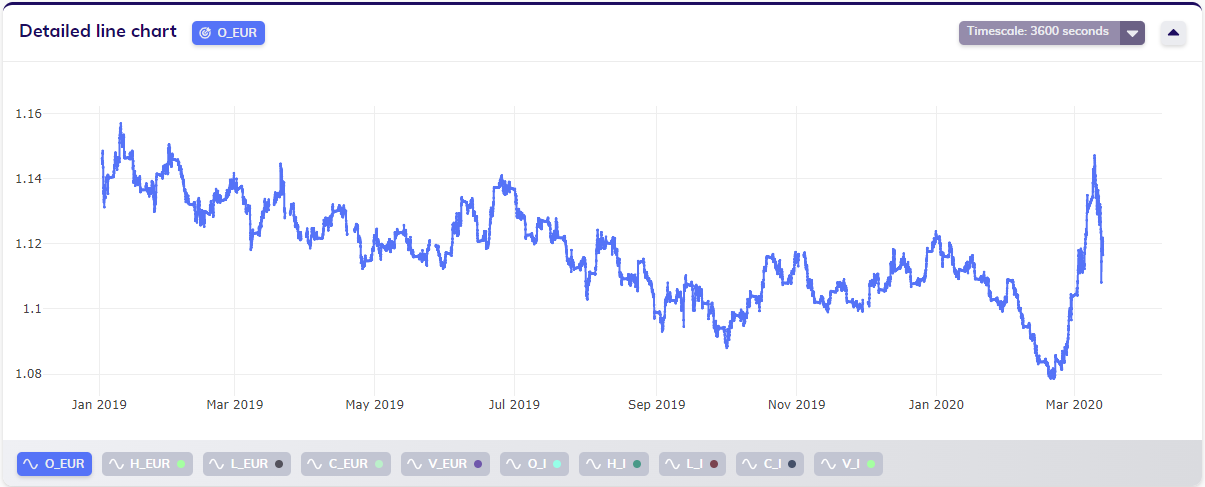
Imagine a user chooses to impute this data, and selects the linear imputation type. To be on the safe side, the user sets the maximum imputation length to 50 samples, covering a little more than a weekend. The result would be the dataset shown below, where most of the gaps are imputed.

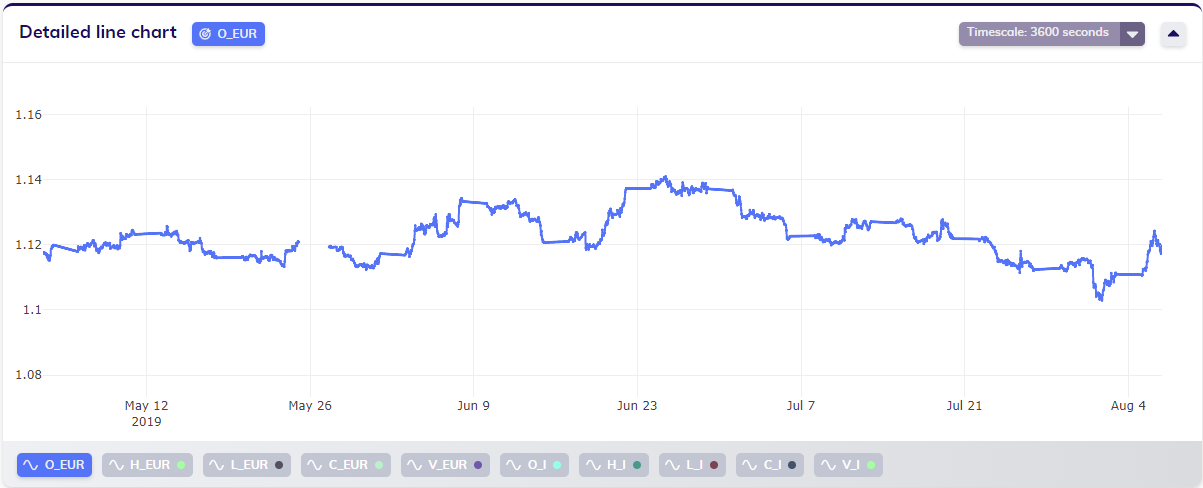
Zooming in on the imputed data shows that most of the weekends indeed show a linear imputation. Around May 26th, 2019, a clear gap is still visible. Looking at the data in more detail shows that the last available observation before the gap corresponds to May 24th, 2019 at 23:00, while the first available observation after the gap corresponds to May 27th, 2019 at 13:00. This indeeds corresponds to a gap of 61 hours or samples, which exceeds the maximum gap length of 50 samples that was set by the user. This alerts the user that on May 27th, 2019, which was a Monday, for some reason no data is available until the afternoon.

Outliers

Sometimes the data may contain observable outliers when something unusual happened - examples include electricity shortages, portfolio changes and breakdown of measuring sensors. In these cases, it might be beneficial to omit the respective observations (timestamps) and the data connected to them, as the outliers may cause the model to be distorted. This only applies to forecasting purposes; in anomaly detection finding these outliers is the exact purpose of the model.

Omiting these observations artificially introduces missing values in the dataset. These can be handled as any other missing values afterwards, and can thus be imputed if desired.