Timescale and Aggregation

Sometimes, the format of the data that serves as the start of a use case doesn't actually match the desired format of the results. These situations require data transformations(s), molding the data to match the expectations and wishes of the use case.

Timescale

Each dataset uploaded to the TIM Repository has a certain sampling period. Sometimes, it may be desirable to scale the data over time, so that the data can be worked with in another granularity than the original (estimated) sampling period. This timescaling also kicks in when regularizing irregular data to make it more suitable for analysis.

For example, IoT data can be measured with a sampling period of one second, while it might be more useful to analyze this data on a more coarse-grained level, such as with a sampling period of a minute or even 10 minutes. Alternatively, sales data might be collected for each hour, while a use case intended to forecast demand to enable adequate restocking is interested in the expected daily or even weekly sales numbers. In such cases, transforming the data by timescaling enables users to intuitively perform their analysis with TIM.

Requirements

The timescale is configured by setting the base unit (second, minute, hour or day) and the number of base units (an integer larger than 0) corresponding to the desired sampling period.

There are certain limits on the available sampling rates to transform data to by timescaling:

• the timescale should not be smaller than the original (estimated) sampling period, and
• the timescale should always be a divisor or product of a time unit.

It is for example possible to set the timescale for a dataset with an original sampling period of 1 hour to 8 hours, or 48 hours (equivalent to setting it to 2 days), but it's not possible to set it to 7 hours or 49 hours.

Aggregation

When scaling time-series data and thereby increasing the sampling period, the data is aggregated in some way. This means that a variable's values over multiple observations are grouped together and condensed into a single value.

Aggregation types

TIM supports multiple ways of aggregating data, including:

• Mean: the mean of the aggregated values is taken,
• Sum: the sum of the aggregated values is taken,
• Minimum: the minimum of the aggregated values is taken, and
• Maximum: the maximum of the aggregated values is taken.

Currently, the chosen aggregation type is applied over the complete dataset, i.e. there is no way to differentiate the type of aggregation between different variables.

Imagine a dataset that consists of product sales numbers, and includes temperature data as a potential predictor. It makes sense to aggregate these sales amounts by Sum, yet intuition indicates temperature would better be aggregated by Mean. Separately setting these aggregation types is currently not supported; however this is mathematically not problematic (in regular datasets) in model building as these differences are caught by the model's coefficients.

Default behavior

By default, TIM aggregates numerical variables by Mean, boolean variables by Maximum, and categorical variables by mode (the mode method is only used for categorical variables and can not be set or changed).

Working with time zones

Using TIM's transformation functionalities such as timescale and aggregation increases the importance of correctly handling time zones, specifically when working with sampling periods shorter than one day.

Model building on timescaled and/or aggregated data

TIM uses uploaded datasets to train all models on. As mentioned before, it may sometimes be desirable to work with data in another granularity than the original (estimated) sampling period and/or to work with regularized (originally irregular) data. Therefore, timescale, aggregation and imputation configuration options are also available for model (re)building functionalities, so the models can be trained and validated on transformed data.

Examples

Seeing the power of the data transformation functionalities offers comes easily when looking at some hands-on examples. This section guides the user through different scenarios in which the above functionalities can be especially useful, and how to use them there.

Lowering sampling rate

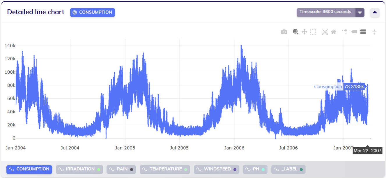
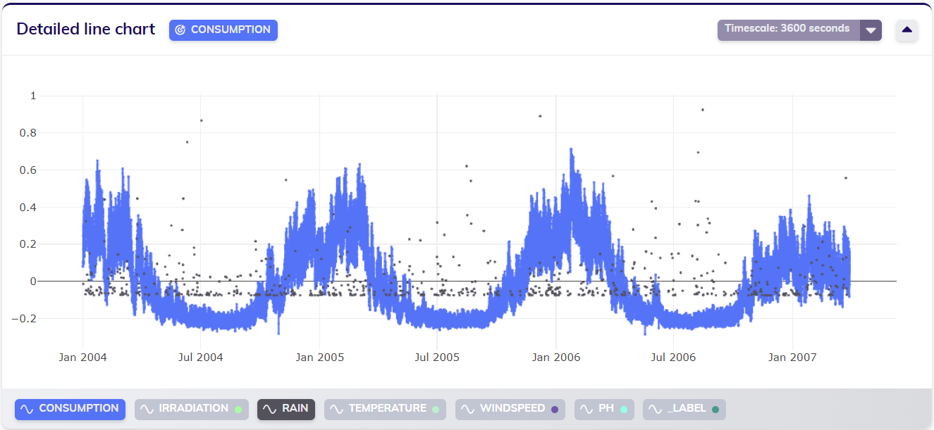
The dataset visualized below has a sampling period of one hour. It describes hourly consumption rates, and contains some additional meteoroligical data as potential predictors or influencers. This data may be measured with an hourly sampling rate because it makes sense to monitor consumption at this rate, and potentially even detect anomalies at this rate.

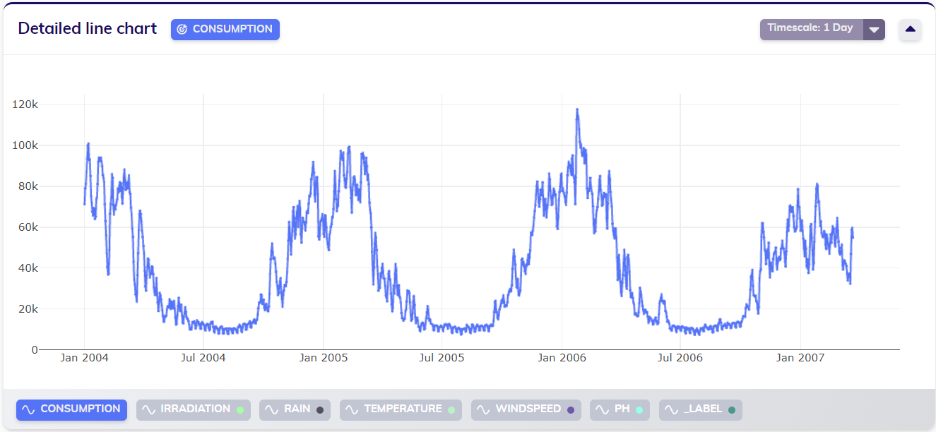
Quite possibly, it doesn't make much sense to forecast expected future consumption on an hourly rate. To prepare for expected consumption, it might very well suffice to know the expected consumption on a daily level. A user may does want to scale this data over time so that it has a daily sampling rate. Applying TIM's timescaling feature for this (with default aggregation) results in the following, rescaled, data.

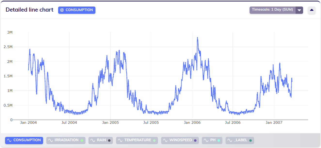
During timescaling as described above, the default aggregation is applied. That means that the (numerical) variables have been aggregated by their mean. For a use case like this, it might make more sense to work with the sum of the consumption over a day, instead of the mean consumption. Combining the timescale and aggregation features allows the user to achieve this. The line chart below visualizes the data (the consumption variable) after doing so. Upon first examination, this may not look very different from the previous line chart (with default aggregation). Closer inspection indicates however that the values in this line chart are of another order of magnitude (200 000 - 3 700 000 compared to 10 000 - 115 000), as clearly visualized on the y-axis. To mathematically inclined people, this might be an indication as to why not seperately setting different aggregation types (mean and sum) for different variables is not an issue for model building (in regular datasets) since the differences will be caught by the model's coefficients.

Regularly missing data

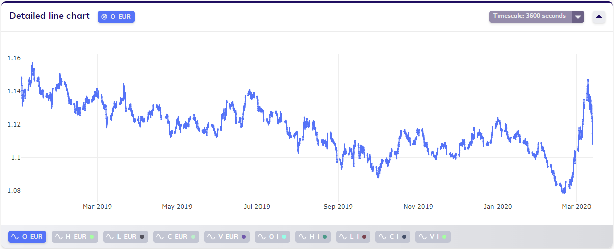
When working with regularly missing data, timescale and aggregation are still available configurations. As an illustration, the following hourly-sampled foreign exchange dataset clearly shows regular gaps.

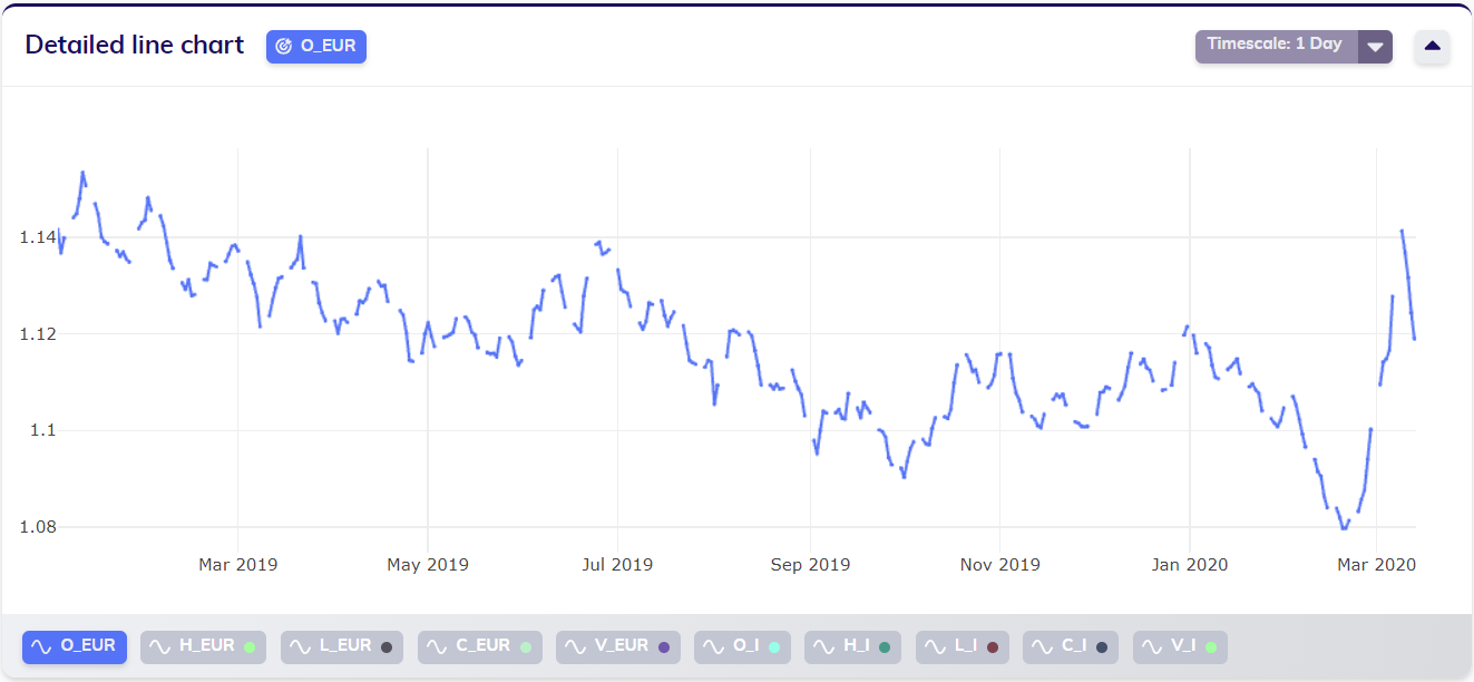
When applying timescale to obtain a daily dataset (with default aggregation), the gaps covering the weekends are still visible in the data (since no imputation was applied in this example).

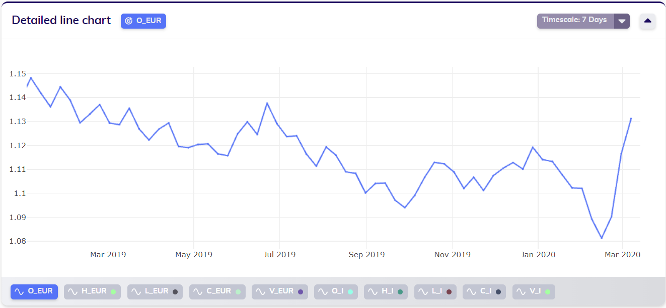
Suppose however that a user wants to work with this data grouped to a weekly sampling rate. In this case, the groups would span over a longer period than the gaps, and consequently there would be no more gaps in the timescaled data. This can also be observed in the line chart below.

Regularizing asynchronous/irregular data

The dataset visualized below is composed of sensor data originating from the monitoring of water quality. Due to the nature of the monitoring the complete dataset is asynchronously sampled, i.e. it consists of irregular data. As displayed above the top right corner of the line chart, TIM estimated the sampling period to be around 900 seconds, or 15 minutes.

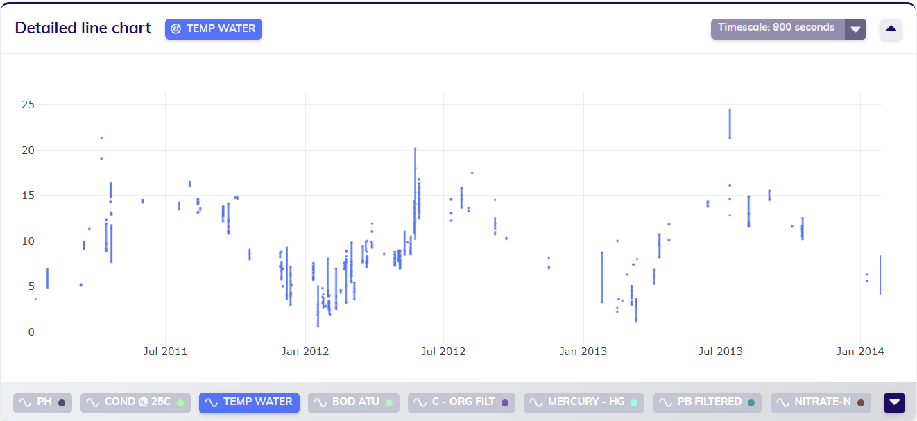
Zooming in to the data shows that TIM already regularized the data to some extend, such that the values are actually displayed with a sampling period of 15 minutes. Missing values are still present though, and this regularization is mainly meant to aide in data analysis.

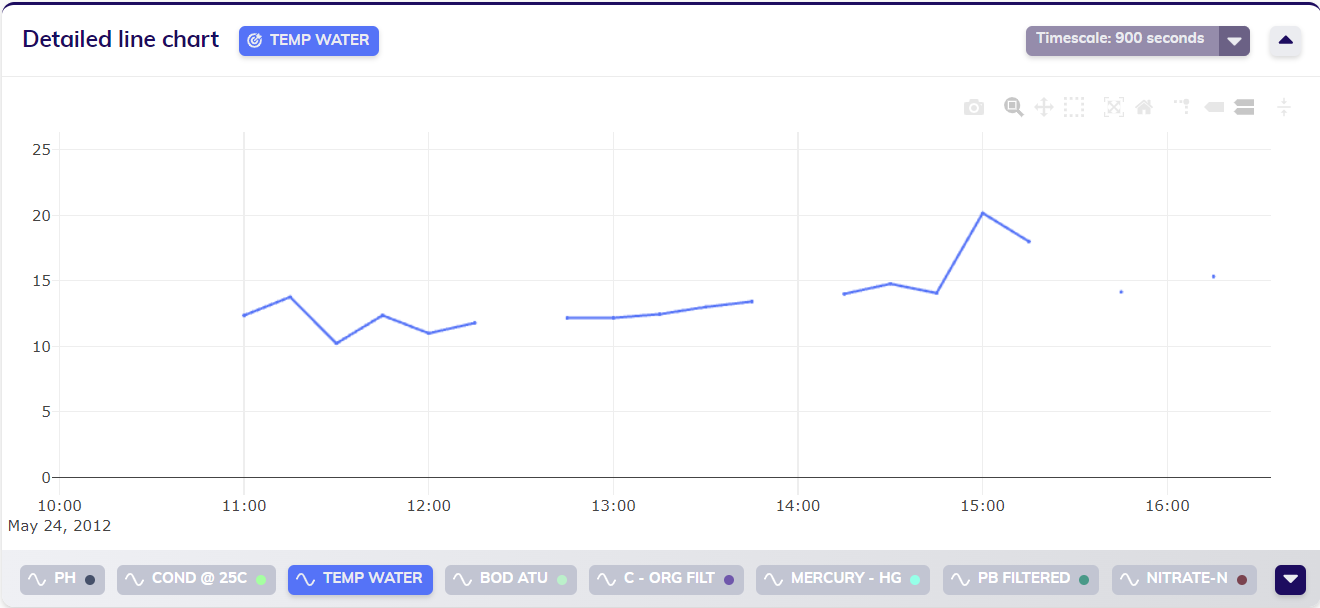
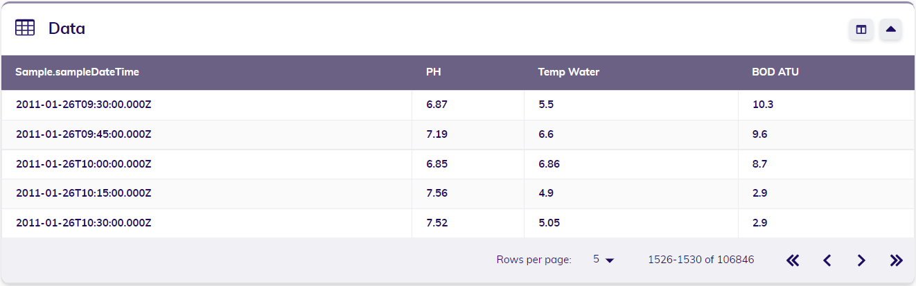
When looking at some of the observations in table format, this can also clearly be seen from the timestamps.

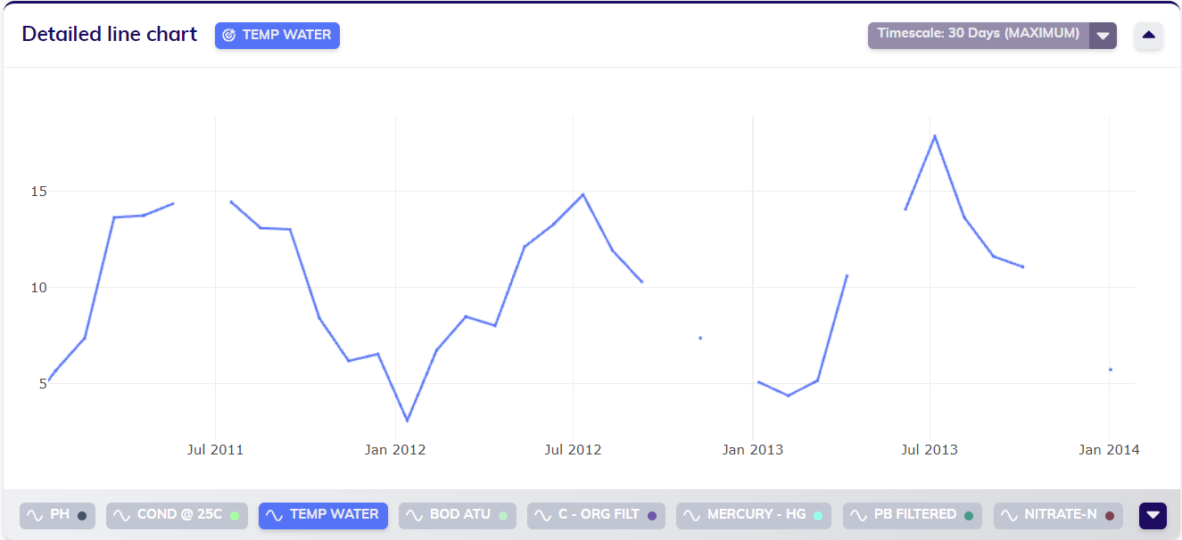
The data is still fairly sparse though, as can be observed from the first line chart above. Using the timescale and aggregation features can be a great start in analyzing this data. From the first line chart, a pattern seems to be emerging over time where the water temperature is lower during winter months and warmer during summer months. Timescaling this data to a sampling period of about a month - 30 days - and aggregating it by maximum (to look at the highest measured values) achieves a result as shown in the line chart below, clearly confirming the pattern seen in the initial line chart.

Combining different sampling periods

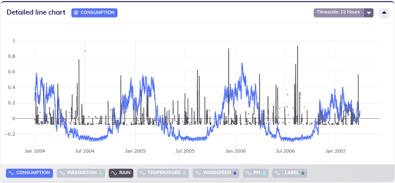
Let us return to the consumption dataset from the first example, as visualized below. This dataset has a sampling period of one hour - at least, the target variable Consumption does.

Selecting the Rain variable and normalizing the data to account for the different orders of magnitude in value of Consumption and Rain shows that the Rain variable does not seem to be measured at the same rate. Looking at the data in more detail verifies this assumption: the Rain variable has a sampling period of 12 hours.

Although TIM supports working with different sampling periods in one dataset, some applications do not. It might very well be the case that a user wants to work with this data in a tabular format, without sparse variables (such as Rain) present. In this case, applying timescale to group the entire dataset on the largest sampling period (in this example, 12 hours) allows the user to do just that. The line chart below displays the same data, timescaled to 12 hours with default aggregation.