Heat Consumption
Problem Description
In this use case, heat is delivered by water. Water heating is a heat transfer process that uses an energy source to heat water above its initial temperature. Typical domestic uses of hot water include cooking, bathing, and space heating. The water is heated in a boiler using fuel (gas, oil or coal) and driven through the pipe by water pumps. Thus, energy is consumed.
As ensuring energy efficiency is of significant importance, it is vital to ask: “Is the consumed energy/heat consumption appropriate under the given circumstances?”. And if not, "What are the possible explanations behind this inadequacy?" This use case highlights the importance of continuous monitoring of heating system health and root cause analysis.
The goal is to automate data interpretation to deliver actionable maintenance recommendations. Concretely, there are 89 buildings, each of them having the consumption of energy/heat of that given building as KPI. The influencers are metered data like the temperatures of incoming and outgoing water flow, the amount of water flowing through the pipe and meteorological data like the outside temperature, wind speed and wind direction. In case of suspicious behavior of the heat consumption of any building, there should be an alert; knowing when something abnormal is happening allows doing inspections in the correct city, of the proper building, and at the right time.
Data Recommendation
The heat consumption of a building is dependent on the outside temperature, the number of people in the building, type of day, and all possible metered variables coming from components of a given heating system. Also, the purpose of a given building may play a role.
In the anomaly detection tasks with defined KPI - like this one, we recommend to include predictors, that are in a relationship with the given KPI. The more influential variables are at your disposal, the better estimation of normal behavior you get. In fact, you have to work with what you have, concerning what is your goal, taking into account other circumstances. A good illustration is wind direction.
If you have a wind turbine that can turn the head so that the blades face the wind through wind direction sensor combined with a motorised head moving mechanism, then wind direction has almost no influence on produces energy of a turbine. In reverse, if there were no such mechanism, wind direction would be crucial to do reasonable anomaly detection.
In this case, the KPI is Heat/Energy consumption. As predictors were available meteorological data like outside temperature, wind speed, wind direction and metered data like temperatures of incoming and outgoing water flow, the amount of water flowing through the pipe.
TIM Setup
There are some settings needed to be adjusted. The period in which you want to build your model and period on which you wish to detect anomalies-in this case, they are the same (all data), as data are quite short (440 observations)-so, there is no need to adjust them. Sensitivity to anomalies is set to 1.5, meaning we would like to be alerted in 1.5% of given points/ we are expecting 1.5% of points to be anomalous. Data have a daily grid, and always when new data point came to the database, all predictors are available - it is the default. Of course, there are cases when you have predictors with other updates and availabilities; then you have to adjust them correspondingly.
Regarding math setting, we do not include offsets of KPI/target - Heat consumption, as we want to detect anomalies only following the meteorological situation and metered values of the system. We also add a monthly perspective- data are changing dynamically throughout a year ( in summer water is not used for heating). In case you are not satisfied with math settings, you can adjust them manually. Documentation for Routine definition and Math Settings you can read in Anomaly Detection section.
Demo example
This section serves as an instruction on how to replicate this problem with TIM Studio and TIM Python Client. Download the data by clicking on the download link.
Target
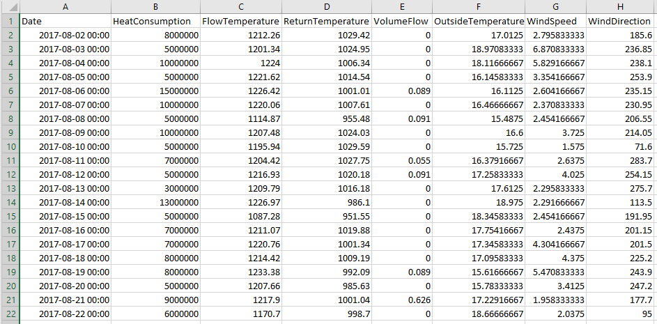
Data used in this example are assembled from a building in the Netherlands. Heat consumption of this building is our KPI/target. It is the second column in CSV file, right after column with timestamps. In this case, the name of the target is HeatConsumption. The data has a daily sampling rate.
Predictor candidates
As predictors, we use flow temperature, return temperature, volume flow, outside temperature, wind speed and wind direction. Thus, for both model building and detection, historical actuals of meteorological and metered data are used. As the same historical data would be available in the daily operational mode, it is a representative simulation.
Data used in this example are from 2017-08-02 00:00:00 to 2018-10-25 00:00:00
Detection scenario
We simulate the real-time detection scenario. Is such a situation, we wish to make detection as often as new data comes into a database. As both KPI and predictors are updating on a daily basis, we do a detection every day. Thus, this scenario does not need to be specially configured; all settings regarding data updates and availability are adjusted by default.
Model building and validation
In this case, both model building and detection are done on the whole dataset, meaning the period from 2017-08-02 00:00:00 to 2018-10-25 00:00:00. Please, bear in mind, detection must not be done for the whole period as it always requires data for calibration when new data range begins – the data are divided into multiple data ranges as they are gappy.
Demonstration
TIM Python Client
After Installation you can use use the notebook and credentials form to run the experiment using TIM Python Client.
Is is also posible to view the notebook.