Error Measures
The goal of error measures is to evaluate the quality of TIM Detect's outputs. Evaluation generally takes all relevant observations into account and compares their anomaly label with the given anomaly score. Thus, to calculate performance metrics, the data needs to be labeled.
TIM returns two metrics: the AUC and the Confusion Matrix.
Visual evaluation
The most straightforward way to judge the performance of a detector is by looking at both the anomaly scores and the labels of the data points in the dataset.
For this intent, analyze the distribution of the scores by creating two histograms, grouped by their label: one illustrates the normal data points, and the other displays the anomalous data points.
Observe the following figure:
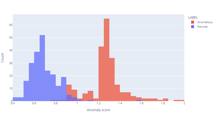
This reveals that in this case, most normal points get assigned an anomaly score between 0.4 and 1 and most anomalous points receive a score between 1 and 2. Since the threshold of determining whether a given data point is anomalous is a score of 1, the anomaly scores nicely separate these two groups and correctly determine which points are abnormal. This also reveals that some anomalous points are in the range 0.4-1 and two normal points can be found in the range 1-2. These points represent false negatives and false positives, respectively.
Histograms are great because they are straightforward to create and interpret, and they contain a lot of information. The performance characteristics are observable through examining this plot, by looking at the capability of anomaly scores to isolate normal states from abnormal ones (and checking out where the average anomaly score falls for both 'classes'), and looking at the level of false positives and false negatives. However, sometimes a user wants to interpret those performance characteristics using quantitative metrics. Such metrics are described in the following sections.
AUC
The goal of the AUC is to represent the ranking ability of anomaly scores. Thus, AUC denotes the probability that TIM will rank a randomly selected anomalous case higher than a randomly selected normal case.
Practically, this tells a user that if they randomly select a normal and an anomalous data point, the anomalous one will have a higher score (indicating a higher likelihood of anomality) with a chance equal to the AUC. This capability is vital in TIM Detect, as TIM tries to ensure that abnormal events get larger anomaly scores than regular events.
The AUC value ranges from 0 to 1. An AUC equal to 1 demonstrates an anomaly scorer that perfectly isolates usual from unusual events. An AUC below 1 means that some normal points have larger scores than some unusual ones (translating into (partly) overlapping histograms). An AUC higher than 0.75 is generally regarded as satisfactory, whereas an AUC of 0.5 means the same level of effectiveness as random guessing.
As an example, the histograms above reflect the following AUC:
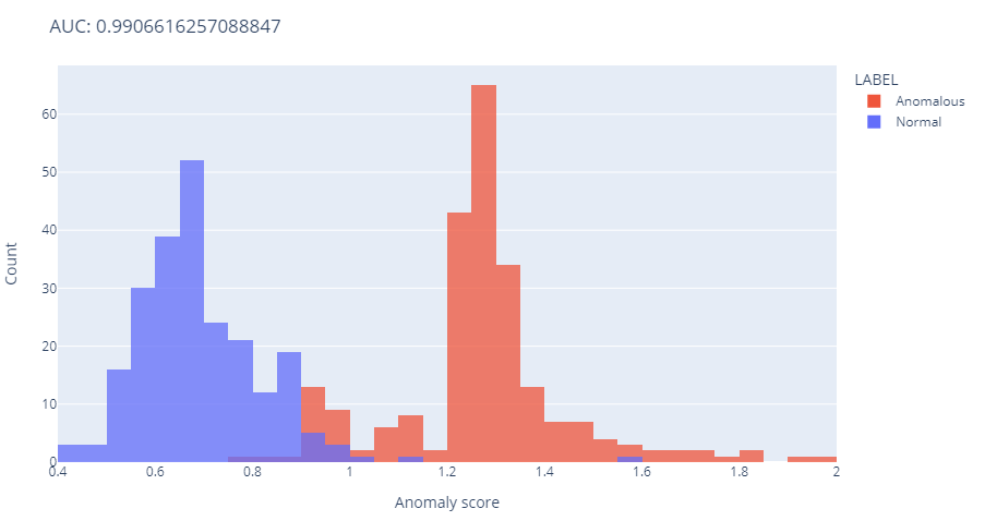
A randomly selected anomalous point will get a higher score than a randomly selected normal point with a probability of about 99 %.
A second example (shown below) represents an AUC of about 0.59:
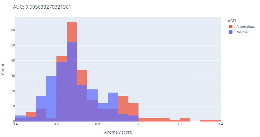
Such results would mean an algorithm cannot differentiate very well between anomalous and normal points, as its effectiveness is only slightly higher than random guessing.
Confusion Matrix
A confusion matrix summarizes a model's ability to identify abnormal and normal points correctly. Computing a confusion matrix can give the user a better idea of what their algorithm is getting right and offers them an understanding of the types of mistakes being made.
The key to the confusion matrix is the number of correct and incorrect prognoses (anomalies) that are summarized with count values and broken down by anomaly label.
As an example, the first figure mentioned above (with AUC of 0.99) corresponds to the following confusion matrix:

In this case, there are 227 data points correctly predicted to be normal (true negatives), 205 data points rightly predicted to be anomalous (true positives), 25 data points points incorrectly predicted to be normal (false negatives), and 3 data points wrongly predicted to be anomalous (false positives).