Features

In the process of expansion, TIM creates many new features from original variables to enhance the final model's performance. This is done through sets of common transformations resulting in new feature dictionaries. After model building, the different features used in the model can be observed in the model's treemap. This section elaborates on the description of these features and how they are obtained.

Identity

PredictorName

The most simple dictionary that takes the data that you provided and filters those predictors that can be used throughout the whole prediction/detection horizon. It is evaluated by taking the exact predictor value for the given timestamp without any time shifts.

This transformation is applied to numerical and boolean variables.

Time Offsets

PredictorName(t - m)

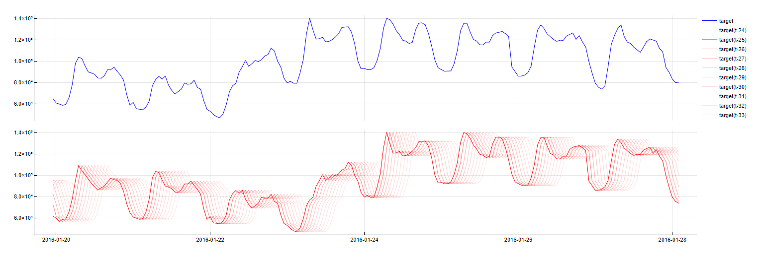
This is easily the most crucial dictionary because it reflects the time dependency of time-series data. A variable in this dictionary is a simple delay/lag/offset in time.

Specific time lags are referred to as a variable's "t-m" delay, in which t represents the time of sample forecasting and m represents the number of time units the lag is removed from t. Note that this might also refer to future values - "t-1" for 12:00 tomorrow refers to 11:00 tomorrow (for hourly sampling rate). This might seem like a slightly contra-intuitive notation because the delay values close to 0 are usually not known. However, for some variables, third-party forecasts are often sufficiently reliable to regard these values as known. An example of this situation can be found in meteorological data. In theory, the upper bound for the time delay does not exist, but in practice, a delay of several time units is usually sufficient. Delay 0 is not considered as the Identity dictionary already takes care of it.

This transformation is applied to numerical and boolean variables.

To obtain this transformation, the variable's timestamp is simply evaluated for the predictor with name PredictorName from m samples ago. Charts below illustrate this concept by showing a signal alongside its time lags.

Weekday

DoW(t - m) = NameOfDay

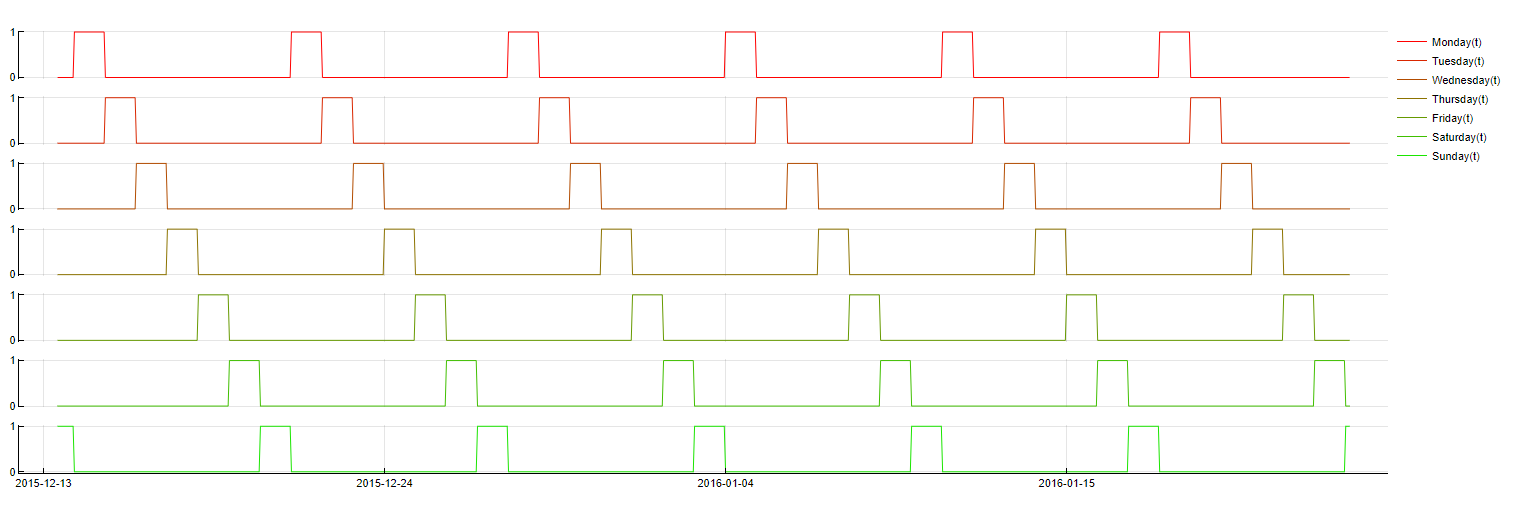
Sometimes a target variable behaves differently depending on the specific day. The sales of a retail store are an example of this scenario. Therefore it is often useful to include Boolean variables representing the different days of the week as predictors. This means variables are constructed with a value of 1 for observations with a timestamp indicating the specific day and a value of 0 otherwise. Often lagged values of these predictors should also be taken into account for optimal performance. TIM currently does not use this dictionary by default, but you can turn it on as "Exact day of week".

To obtain this feature, the following simple logic is used: if the timestamp from m samples ago belongs to NameOfDay, the value of 1.0 taken, otherwise, the value of 0.0 is taken. The graph below shows the value of each weekday indicator over time.

Weekrest

DoW(t - m) ≤ NameOfDay

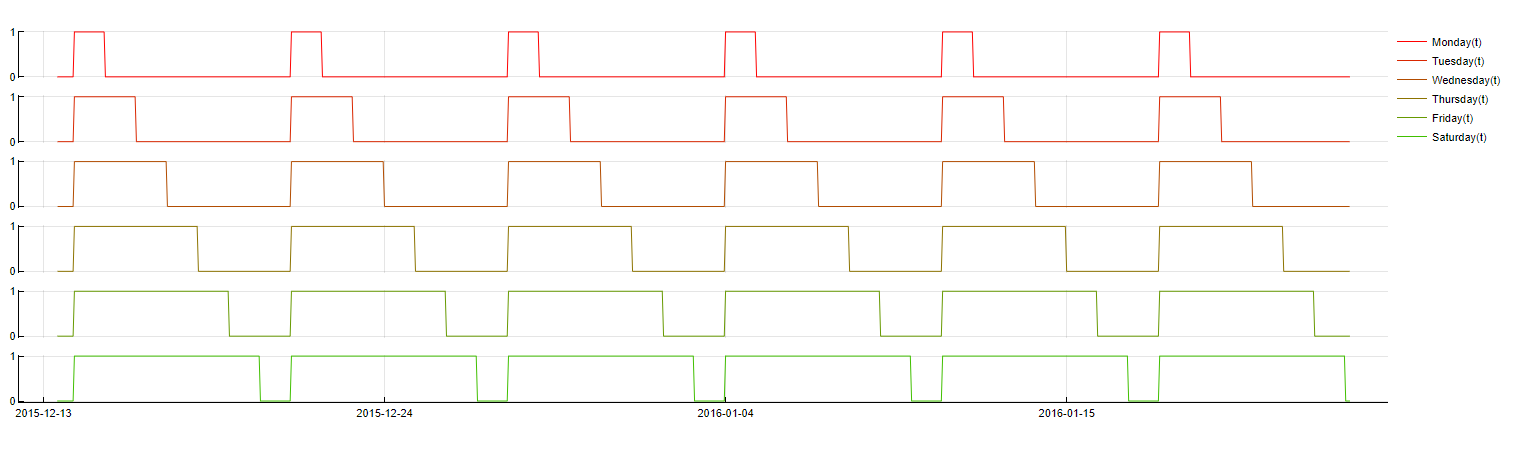
It is sometimes beneficial to exchange weekday dictionaries for what so-called weekrest dictionaries, whose construction is slightly different. Whereas weekday transformations ask whether a timestamp belongs to a certain day, weekrest transformations ask whether a timestamp belongs to one of several days; for example: "Does this timestamp belong to either a Monday, a Tuesday or a Wednesday?" These transformations tend to be more robust and can eliminate redundant computation time. However, their interpretability is more complicated. By default, TIM uses a Weekrest dictionary.

To evaluate this feature, the following logic is used: if the timestamp from m samples ago belongs to any of the relevant days, the value of 1 is taken, otherwise, the value of 0.0 is taken. The graph below shows the value of each weekrest indicator over time.

Month

Month ≤ NameOfMonth

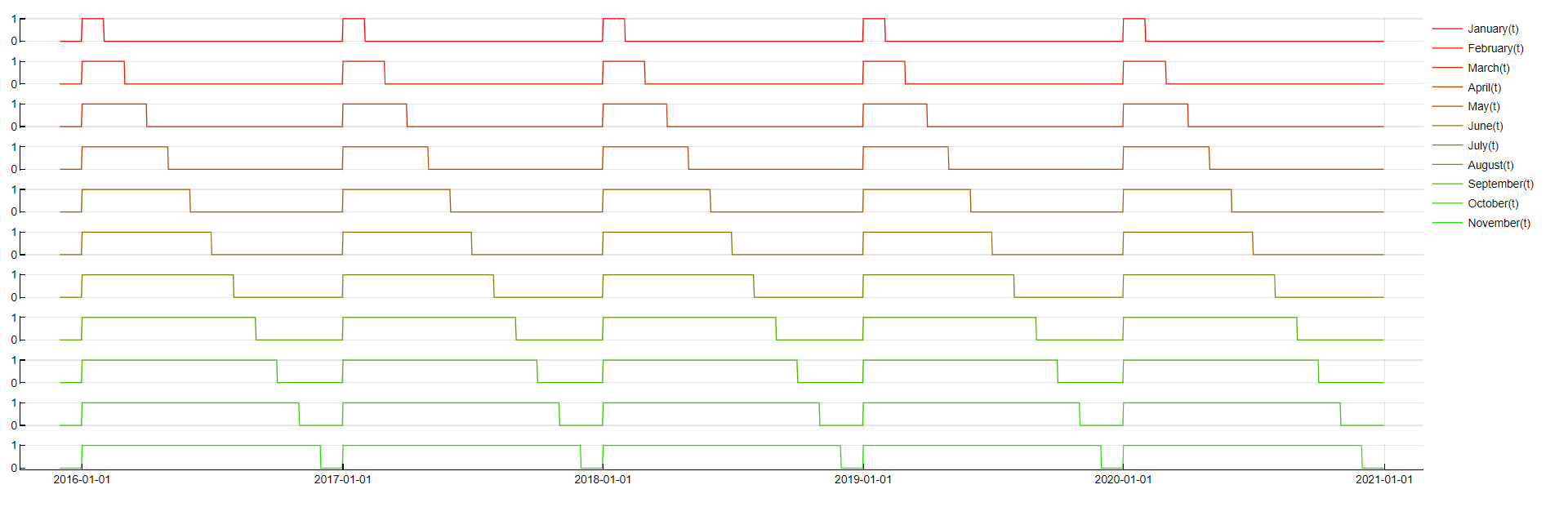
For reasons similar to the reasons for using the weekrest dictionary we could also use a dictionary tracking month of the year. However, this dictionary usually does not improve the accuracy at all because there mostly are not enough distinct months to be relied on. In some situations, it still might make sense to use it though. To make it more stable we use the "rest" (see above) version and do not use time lags.

To evaluate this feature, the following logic is used: if the timestamp belongs to any of the relevant months, the value of 1 is taken, otherwise, the value of 0.0 is taken. The graph below shows the value of each month indicator over time.

Public Holidays

• PublicHoliday(t - m)
• PublicHoliday(t + m)

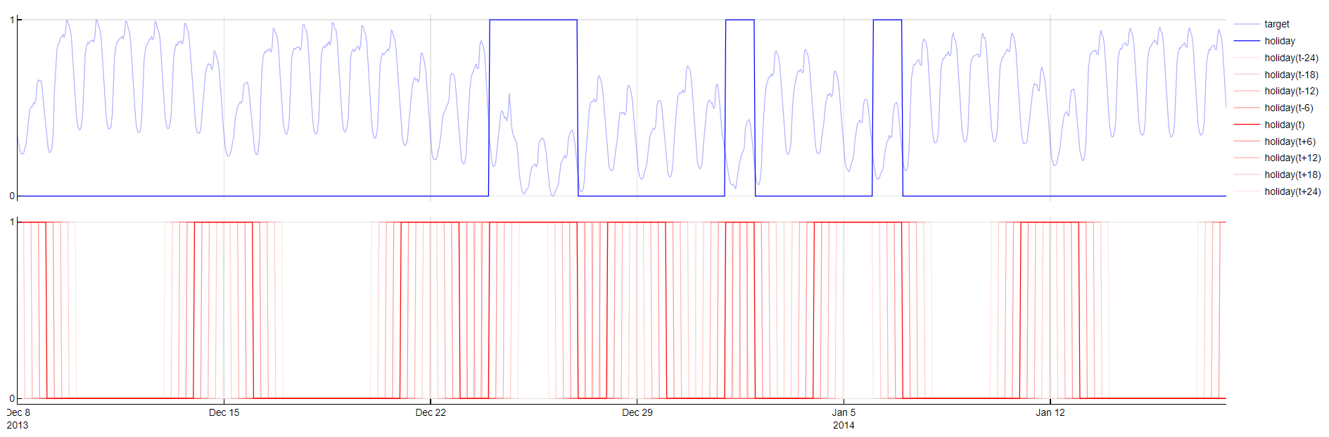
Sometimes a target variable behaves differently during working and non-working days. Non-working days include weekends and public holidays. To capture these effects Public Holidays dictionary creates new variable which contains 1 if a time-stamp is Saturday, Sunday or public holiday given by user. Inclusion of weekends to public holidays enlarges training set of non-working days since there are only a few public holidays during a year. Days before, after or in between non-working days usually have specific behavior as well, e.g. bridge days. Therefore this dictionary generates negative and positive time-lags of the new variable. Since this dictionary uses positive time-lags, public holidays should be provided for one day ahead than forecast horizon is. Predictor public holidays given by user should contain 1 for public holidays and 0 for other days. To use this dictionary the predictor has to be marked with predictor type Holiday.

This transformation is applied to boolean variables and only one boolean variable can be selected as the holidayColumn in the configuration.

To evaluate this feature, the following logic is used: if the timestamp from m samples ago/ahead is either public holiday given by user, Saturday or Sunday, the value of 1.0 is taken, otherwise, the value of 0.0 is taken. The graph below shows values of public holiday predictor given by user and its transformations created by TIM.

Periodic decomposition

• Sin(period, unit)
• Cos(period, unit)

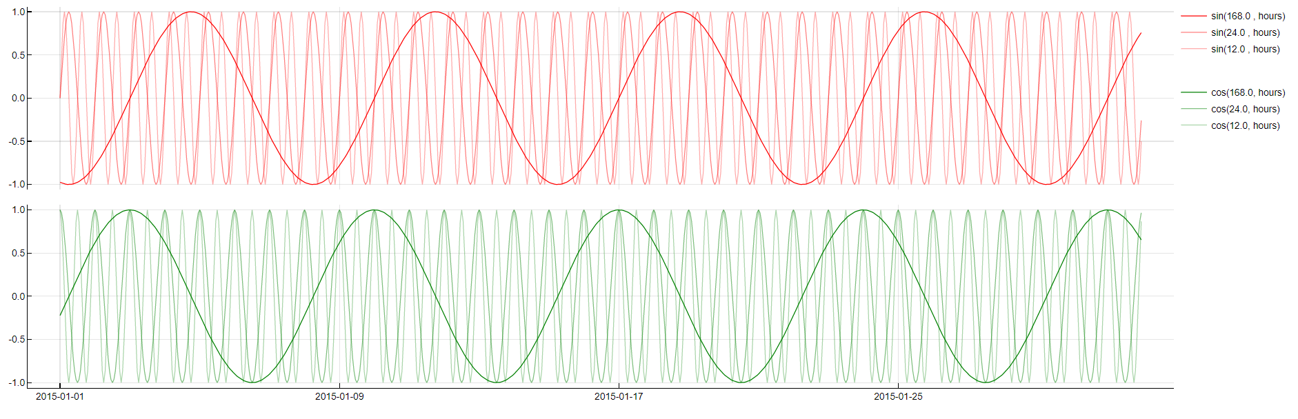
Humans tend to behave in cycles. Whether it is a daily cycle, a weekly cycle (such as represented by the weekdays dictionary) or something more uncommon, it often benefits performance to identify these cycles, their phases and their periods and incorporate corresponding variables in the models. The best tool for such a decomposition is called FFT (Fast Fourier Transform). In reality, most business problems tend to exhibit the same periodic cycles. Therefore, it is reasonable to focus amplitude search to the most common amplitudes (namely 24, 12, 6, and 168 for 24-hour granularity). API 4.1 had phases in sines as well, since 4.2 they are omitted.

To obtain this transformation the following formula is used: sin(epoch* 2π / period), where epoch is the number of time samples since year 0 (up until this specific timestamp) with a given sampling rate. The following graphs visualize a target signal accompanied by a sample of sine waves with daily and weekly period which enter the search for the best period candidates.

Fourier

Fourier(period)

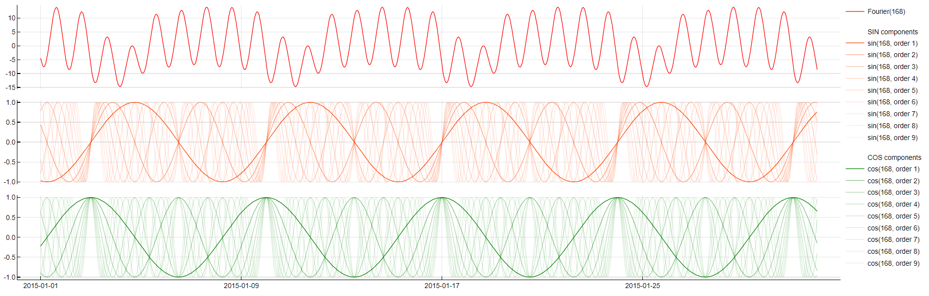
Those who studied math probably know that there are more deep rooted mathematical reasons for using sine waves to model time series. The whole signal can be decomposed by using only sine and cosine waves by a so called "Fourier Transformation". While in the periodic dictionary TIM lets partial sine waves loose to potentially combine and interact with other predictors, this dictionary puts all signals together to form a good approximation of the target itself. This might be beneficial for time series that are better modeled without time lags or have too few observations.

To obtain this transformation TIM linearly combines all partial coefficients of all sine and cosine waves stored in the model under the period tag. As there are usually too many, we do not display them in the treemap.

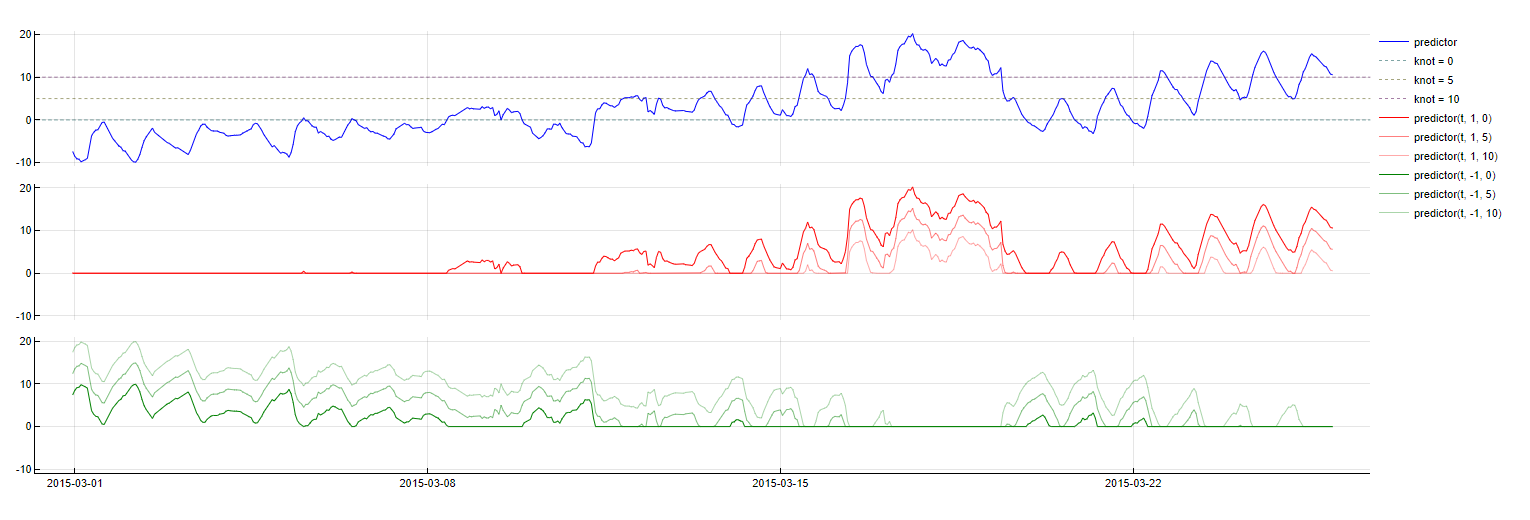
Piecewise Linearity

• max(0, knot - PredictorName(t - m))
• max(0, PredictorName(t - m) - knot)

This transformation essentially splits a variable into different working regimes and enables TIM to fit different regression coefficients to each of those regimes - resembling a piecewise linear polynomial fit. This improves performance when the dependency between a predictor and the target variable is nonlinear. All of these transformations can be lagged over time as well; TIM therefore works to find a relevant knot as well as a relevant time lag.

This transformation is applied only to numerical variables.

To obtain this transformation the formula max(0.0, type * (lag - knot)) is used, where lag is the value of the predictor PredictorName from m time units ago and type has two possible values, namely +1 and -1. The following graph shows the transformation for both types with a sample of three knots.

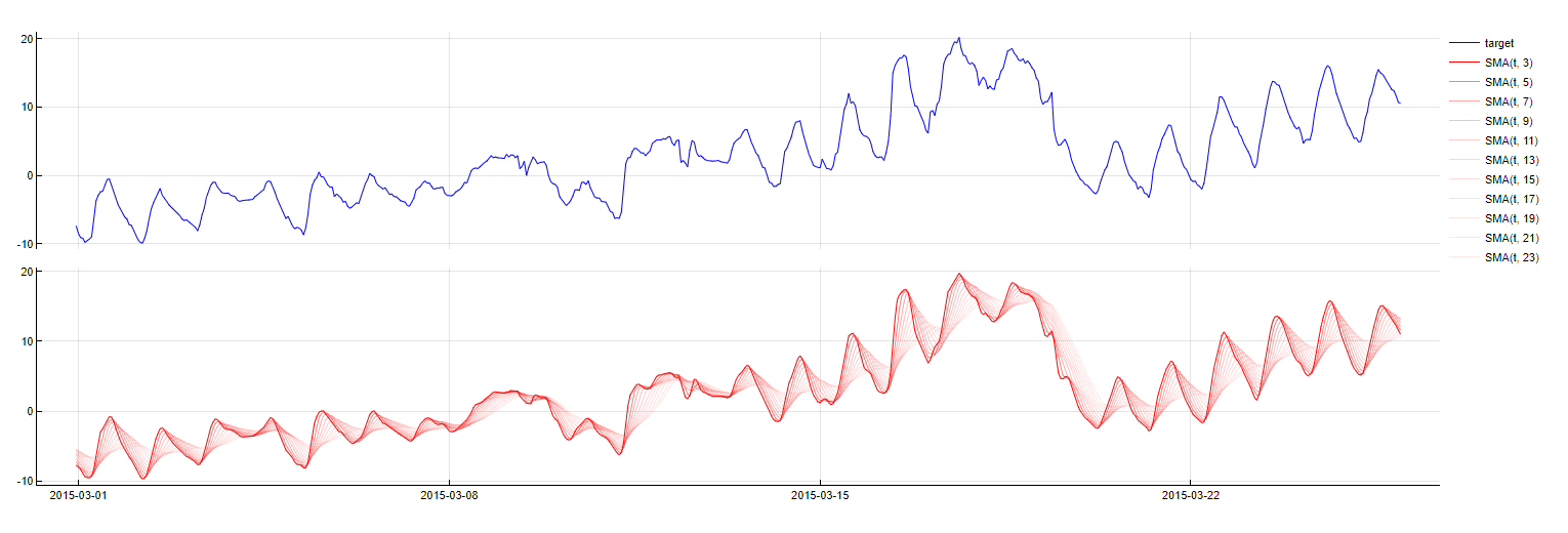
Simple Moving Average

SMA_PredictorName(t - m, w = window)

This dictionary creates simple moving averages, i.e. signals that copy the average of target or predictors with a certain delay and within a certain computation window. This helps keep track of long term high scale changes in the signal and uses weights for other variables to compensate these higher scale changes. The parameter space for this transformation is two-dimensional, as it includes a relevant time lag as well as an optimal computation window.

To obtain this transformation, the mean of the values of the predictor variable within the specified window are calculated, exactly up to the timestamp m samples before the timestamp being evaluated. The graphs below show a signal accompanied by its simple moving average calculated with different window lengths.

This transformation is applied only to numerical variables.

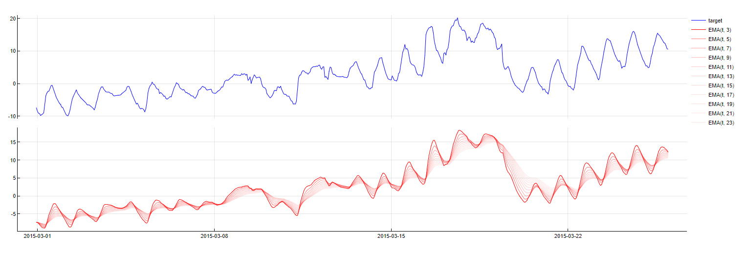
Exponential Moving Average

EMA_PredictorName(t - m, w = window)

This dictionary is similar to the Simple Moving Average dictionary but places greater significance to the most recent data points. This technique creates a weighted average of the most recent target value and the most recent (i.e. the previous) exponential moving average itself. Instead of looking for an optimal window length, TIM looks for an optimal weight value. This type of transformation involves a certain risk as it takes some time to "calibrate", i.e. to stop focusing on the initial input values. Therefore, this technique cannot be used when forecasting without sufficient amount of calibration data, as the result would be misleading - TIM uses SMA in these cases instead. Currently, TIM applies this transformation to the target variable only.

To obtain this transformation, it is necessary to calculate the exponential moving average for all target data points starting from the first one up to the the timestamp m steps before the that is being evaluated. This is done through a recurrent relationship: EMA(t+1) = (1 - α)EMA(t) + αtarget(t) where α is 1/(1+window). The following graphs show a signal accompanied by its exponential moving average calculated with different window lengths.

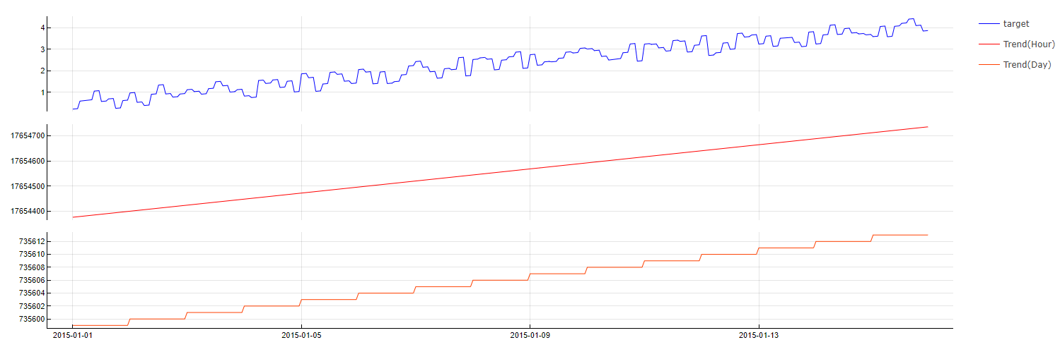
Trend

Trend(step)

TIM does not need a trend variable by default, because it usually relies on using time lags of the target variable itself, which carries the changing trend information within. However, sometimes it might be interesting to amplify this effect even more or use it when time lags of the target cannot be used. The step of the trend may be Second, Minute, Hour, Day, Month or Year. The values are constant in the dictionary during this step period. TIM only selects trends with the most suitable steps.

To evaluate this dictionary, the timestamp is converted into the number of steps from the date 0000-00-00 00:00:00.000.

One-Hot Encoding

PredictorName(t - m) = category

This transformation is used to transform categorical variables into a format that can be used in the model-building process. It works by creating new binary columns, where each column corresponds to a unique category of the original categorical variable. If a data point belongs to a particular category, the corresponding binary column will be set to 1, and all other binary columns will be set to 0. If the predictor is known for the entire prediction horizon, no time lag of the predictor is used (m = 0). Otherwise, the closest possible time lag is used.

Note that this transformation can result in a large number of predictors if the original categorical variable has many unique categories. Therefore, TIM does not apply this transformation for predictors with more than 20 categories.

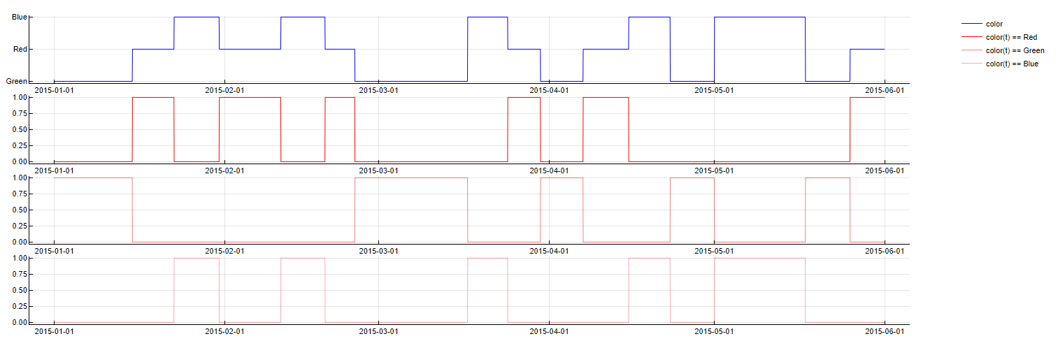
To evaluate this transformation, the value of the predictor named PredictorName from m samples ago is compared with the specified category value. If they match, 1 is returned; otherwise, 0 is returned.

Polynomial

transformation1 & transformation2

Some predictors behave differently depending on the value of other predictors. For example, a person might consider going to a park when the weather is sunny, but only in case he/she does not have to work that day. The best suited mathematical operation to model this kind of interaction between different variables is a simple product. The polynomial dictionary looks at these interactions by assembling products of predictors (element-wise products of two vectors). In theory, all predictors could be combined into very large polynomial expressions of higher degrees. In reality, however, second-degree expressions are sufficient most of the time. TIM avoids interactions of vectors with themselves (squares), as they do not tend to improve model quality. This dictionary is applied last, so it is able to combine features from all previous dictionaries.

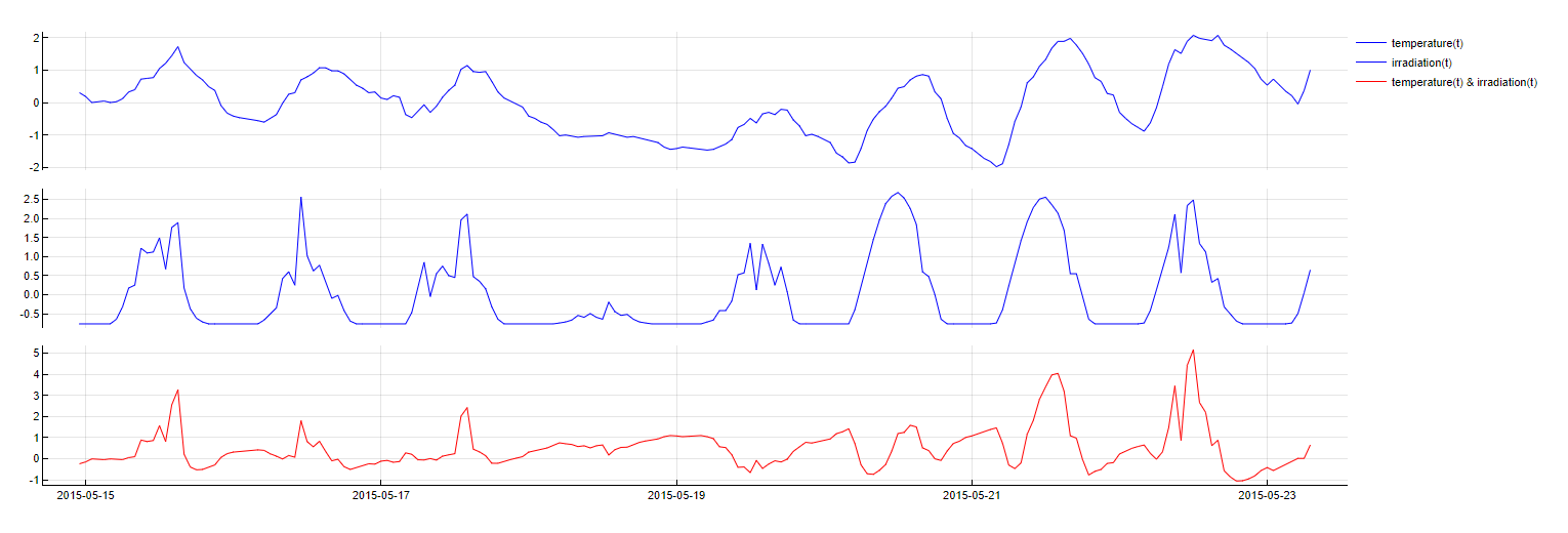
To obtain this transformation, two predictors are simply multiplied. The graphs below show two predictors (irradiation and temperature) as well as their interaction.

Intercept

Intercept

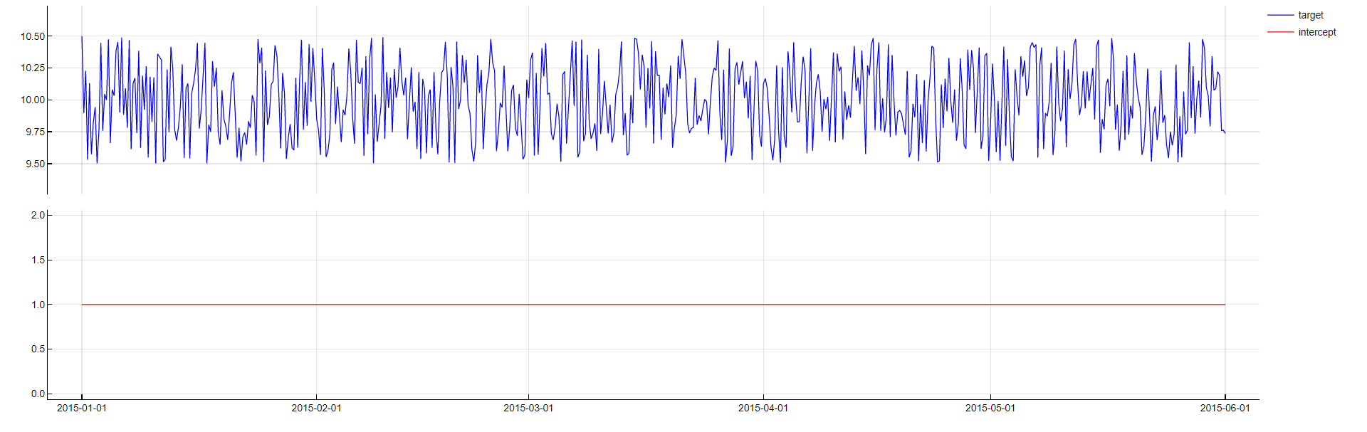
Including an intercept in a model is very easy to do, but can greatly improve performance. This is done by including a vector that is used to express the mean of the target variable and help the modeling process.

Including an intercept in a model is simply done by including a vector containing different instances of the value 1.0.