Time-series Forecasting
Time series provide a completely different challenge than other ML tasks. In order to successfully make forecasts based on time-series data, it is important to understand where the differences come from and how they can be exploited to create a fully automated modelling engine. On this page, some critical aspects of time series modelling are demonstrated using simple examples.
More data, more problems
In the following images, two completely different signals are visualized. The first signal describes gas consumption and the second image is an aggregation of different electricity consumptions. They do, however, have one thing in common: structural changes. A structural change can present itself in many ways, such as a change in mean, variance and/or seasonality. Sometimes the change is so fundamental, that it effectively seems to split the time series in several different time series.

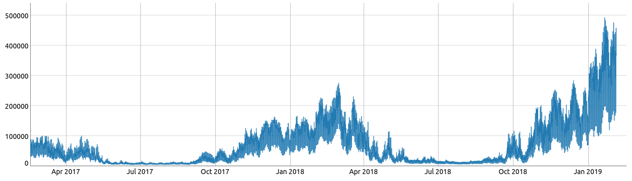
When trying to teach ML algorithms on how to play Go or how to distinguish between pictures of lungs to detect lung cancer, more data samples typically enhance performance. This, in general, is not the case when modelling time series. A large dataset might contain data from both before and after a particular structural change, making it harder to make correct forecasts if the structural change is not correctly recognized. Even more tedious, after a structural change, new data might suddenly render a previous model useless. However, this aspect of time series modelling can also prove to be an advantage sometimes, because it usually eliminates the need to deal with enormous datasets containing millions of records. In conclusion, it is crucial to learn when and with what data time series models should be (re)trained.
The data ordering
When dealing with time series, the time ordering of the data is crucial. This is different from other data types, where the order of the dataset does not matter. Time series are often even cross-correlated, meaning that the value of the target variable at time t (partly) depends on values of predictors from times t-k. This is unpleasant because new data is not immediately available.
The arrival of data samples might even be completely asynchronous, causing models using values from specific time lags to become useless if this data is not available when making a forecast. It is important always to consider this when modelling time series. Another way to overcome this problem would be to retrain the model every time a new forecast needs to be made. It is, however, nearly impossible to do so with AutoML techniques, due to the long time needed to build models.
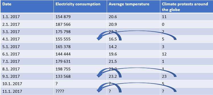
Consider the dataset below. The goal is to predict electricity consumption, which leads to the following model:
Electricity consumption (t) = 10000 ∙ Average temperature (t) - 5000 ∙ Protests (t)
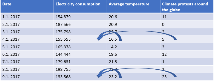
If you want to use the calculated model to forecast future electricity consumption, this model becomes useless. As both temperature and the amount of protests are not available yet, they cannot be used for forecasting purposes. (On January 10th, if you wish to forecast electricity consumption for January 11th, your model is useless.)
Making multiple predictions
In practical use cases, it is rarely the case the only forecast is desired. Most of the academic research focuses on the algorithm in use, but then tends to use this algorithm to make one single forecast. This is very different from typical business use, where multiple forecasts over multiple different time spans are needed.
Typical neural network solutions solve this problem by creating architectures with multiple outputs - for example, 24 outputs when forecasting value for every hour of the next day. However, what happens if a user wants to use this model to make forecasts up to 36 hours ahead? Nothing, as this is simply not possible.
The best way to overcome this obstacle would be to retrain an adjusted model (with 36 outputs), but this takes a considerable amount of time and effort. Moreover, this does not solve the same problem in future situations, as the model is still limited to the fixed anticipated outputs.
Non-linear dependencies
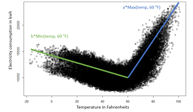
Modeling electricity consumption using temperature values illustrates that the dependency between two variables is not always straightforward. This makes sense: during peak winter and summer time, people tend to consume more electricity due to heating and air conditioning usage. Both low and high temperatures thus lead to higher electricity consumption.
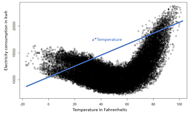
This means that the dependency of electricity consumption on temperature changes depending on the value of the temperature. A linear model, such as the one shown in the figure above, would therefore not be appropriate. However, if it is possible to discover at what temperature value this dependency changes, this problem can be overcome. The temperature predictor can then be separated into two new predictors, as shown in the figure below. This is important because it demonstrates the importance as well as the possibilities of feature engineering.
One might propose to just use a nonlinear model for this dependency, instead of separating the predictor. In this simple example, this is indeed a solution. In more complex situations, however, this might not always be the case. With increasing model complexity required training/learning time also increases, as well as the chance of overfitting the data.
Training multiple simple models might therefore be preferable to training a single very complex model in many different cases. Retraining this very complex model might even become economically unfeasible due to the time it requires and the cost it brings. Still, finding which simple models to include in the final composite model requires decent feature engineering. Moreover, in many industries model explainability is an important requirement for business cases. Simpler models are generally easier to explain than more complex ones, again providing an argument in favor of simpler models. Some complex models are even impossible to explain.
Dependency over time
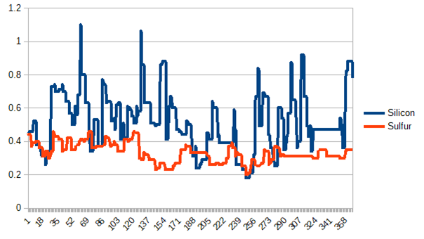
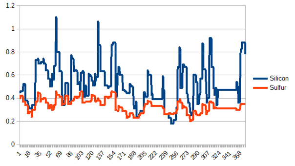
When modelling time series, usage of so-called lags or offsets is crucial. To illustrate why let’s take a closer look at a furnace melting metals. The evolution of the levels of silicon and sulfur in the final product throughout time is measured. In the graph below, both series do not seem to exhibit a strong correlation. However, by offsetting the levels of sulfur by 15 steps, both series suddenly become visibly correlated.
This is also something people should be familiar with when reacting to changes in real life. These changes typically do not show up right away, but with some delay - you will turn the heat up when you find your apartment to be colder, not reacting to the actual outside temperature, but to the one from an hour or two before. This also has consequences for time series modelling, because it once again demonstrates that correct feature engineering matters. Whether you should use a predictor from time t, or t-100, how far back in time you should go, and other related questions are not trivial to solve.
Time to which the forecast applies
Imagine trying to forecast how many cars will be moving into the city an hour from now. At 3:00, the model cars(t)=cars(t-1) would probably produce decent results. There is no reason to believe that the number of moving cars will change suddenly between both times. However, would you use this model at 16:00 to forecast the situation at 17:00? Probably not. The variance is a lot higher during these times. Suddenly other factors come into play, such as the weather. While certain predictors – such as rain – might not be helpful at night, they might be crucial during daytime. Both situations technically consider the same time span, a prediction for one hour ahead, the required model complexity differs a lot.
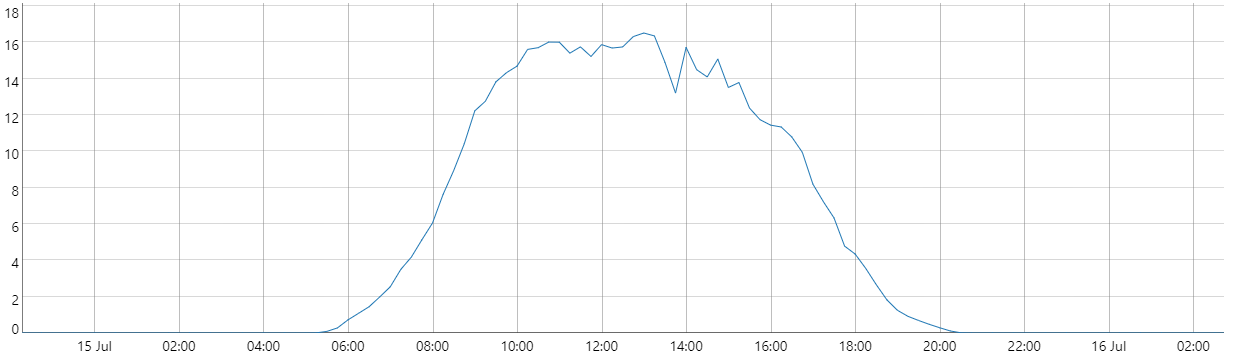
The graph below shows the production of a typical solar farm during one day. Imagine you wanted to forecast this production. To forecast the production at 3:00, the model production(t)=0 probably produces good results; the sun simply does not shine at night. Even so, this model would obviously fail to accurately forecast production at 12:00. Once again, the required model complexity differs a lot, depending on the time for which you want to forecast.
In general, a proper understanding of the ‘situation’ that occurs when forecasting (when and what needs to be forecasted as well as the data availability at the time of forecasting) might drastically improve accuracy, since no complexity is wasted where it is not needed and additional complexity can be provided where it is needed.