Datasets
![]()
Users can upload, preview, manage, and explore datasets in TIM Studio. They will be able to leverage TIM’s time-series database, and TIM Studio will provide users with an overview of metadata and statistics that might be relevant in the data exploration and preparation phase.
The repository also includes version management, allowing you to keep track of your version history and update your datasets as new data becomes available.
The datasets overview
In the datasets overview, a user will find a list of all the datasets they can access. Relevant metadata, such as the workspace and team to which a dataset belongs, the number of observations in the latest version, the variables it contains, the last update, and the time of creation, can be viewed directly from this overview.
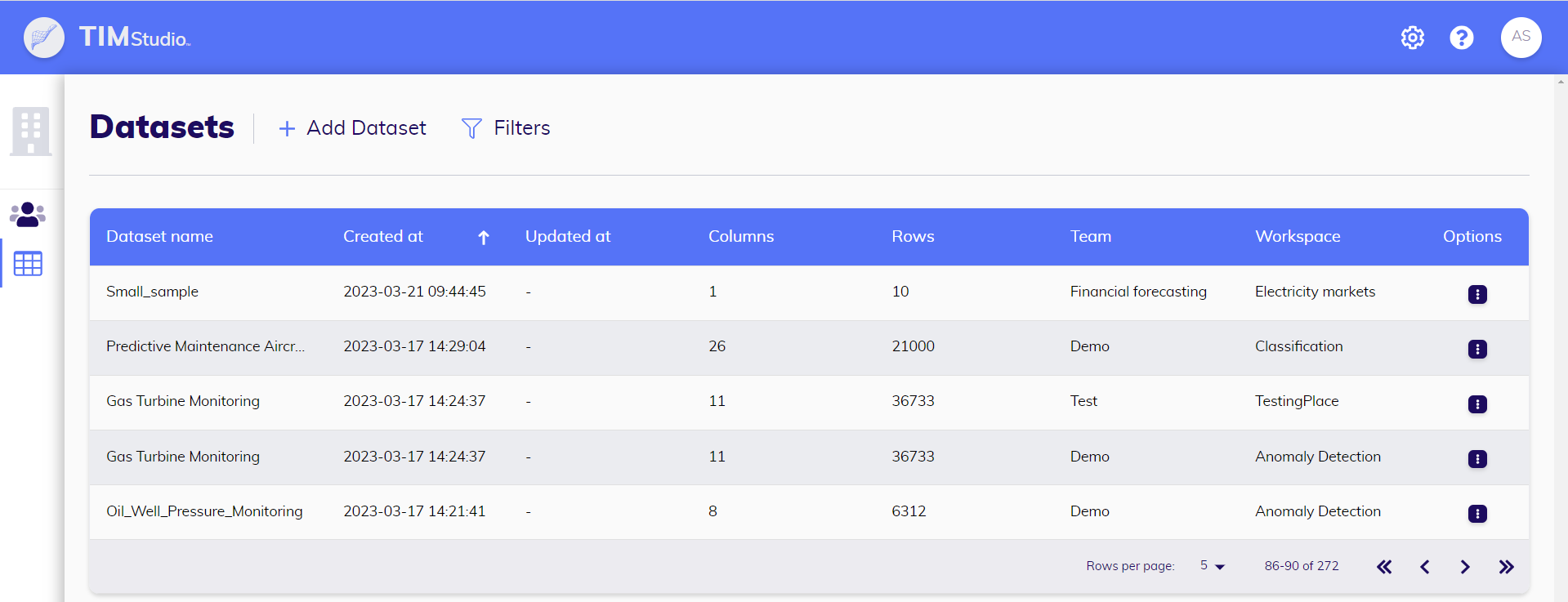
On this page, new datasets can be uploaded, and existing datasets can be downloaded, updated, edited, and deleted. Dataset logs can also be viewed from this page.
Uploading: Uploading a new dataset allows the user to select the data source set the dataset's name and description. During the uploading process, users will get to see a preview of the dataset, allowing them to visually check whether they selected the right dataset and set the correct properties.
- CSV: If the user opts to upload a CSV file, they will be able to set its properties: the column separator, the decimal separator, the timestamp format and the timestamp column). TIM Studio aides the user by recognizing and suggesting a range of timestamp formats, CSV separators and decimal delimitors automatically.
- SQL: If the user opts to connect to an SQL table, they will be able to set the connection properties: the database name, the database type (supported types include PostgreSQL, MySQL, MariaDB and SQL_Server), the host, the user name, the password, the port and the table name.
Downloading: Downloading a dataset allows a user to extract a CSV file containing this dataset, to upload the same dataset in another Workspace, or to be used for any purposes that do not involve TIM Studio.
Updating: Updating a dataset allows the user to upload a new version of an existing dataset, adding new observations or overwriting existing observations. During the updating process, users will get to see a preview of the dataset, enabling them to visually check whether they selected the right dataset and set the correct properties. When updating by uploading a CSV file, TIM Studio will once again aid the user by automatically recognizing and suggesting a range of timestamp formats, CSV separators, and decimal delimiters.
Editing: Editing a dataset allows the user to update its name and its description.
Deleting: Deleting a dataset will also permanently delete all of its versions.
Viewing dataset logs: A dataset's logs contain information about TIM's actions on that database (during uploading and updating) as well as any observations TIM makes (informative as well as warnings), and any errors that may have occurred.
The dataset detail view mode
On a dataset's detail page, you can find all the information regarding the dataset. This includes its name, description, creation date, last update date, estimated sampling period, the number of observations and variables it contains, as well as the available versions of this dataset. The page also features a detailed graph and table, allowing users to explore the data in depth. An overview of the dataset's statistics is provided, including relevant information for each variable (minimum, maximum, and average values, as well as the amount of missing observations). Additionally, to quickly navigate to where the dataset is used in the structure of the TIM repository, the page displays the use cases that center around it.
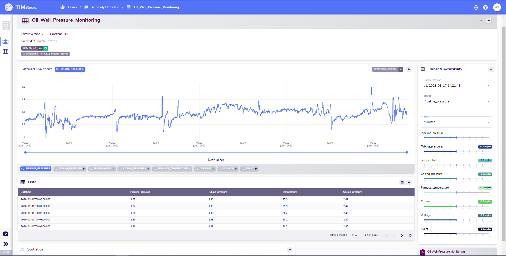
The version pills in the title card give an overview of the available versions of the dataset and their status. These pills are also clickable (when the status is finished or finished with warning), and clicking them will update the page with the data and statistics of the selected version.
From this page, a user can easily browse a specific use case of interest. They can also navigate through the different versions of the dataset. Additionally, a user has the option to update the dataset (i.e., upload a new version), as well as download, edit, and delete the dataset. To begin building models based on this dataset, the user can link an existing use case to this dataset and add a new use case linked to this dataset.
Updating: Updating a dataset allows the user to upload a new version of an existing dataset, adding new observations or overwriting existing observations. During the updating process, users will get to see a preview of the dataset, allowing them to visually check whether they selected the right dataset and set the correct properties. When updating by uploading a CSV file, TIM Studio will again aide the user by recognizing and suggesting a range of timestamp formats, CSV separators and decimal delimitors automatically.
Editing: Editing a dataset allows the user to update its name and its description.
Downloading: Downloading a dataset allows a user to extract a CSV file containing this dataset, to upload the same dataset in another Workspace, or to be used for any purposes that do not involve TIM Studio.
Deleting: Deleting a dataset will also permanently delete all of its versions.
Inspecting variables' availabilities: See the section on the availability component below.
Scaling and aggregating the data: See the section on the timescale component below.
Linking to a use case: Linking a dataset to an existing use case is possible if the relevant workspace contains at least one use case that does not have a linked dataset. By creating this link, the user can start creating experiments and executing jobs in the linked use case.
Adding a linked use case: Adding a use case allows the user to create a new use case that already contains a linked dataset, namely the one that the process was initiated from. This empowers the user to start creating experiments and executing jobs in this newly created use case right away.
Viewing dataset logs: A dataset's logs contain information about TIM's actions on that database (during uploading and updating) as well as any constatations TIM makes (informative as well as warnings), and any errors that may have occured.
Quick forecasting: Quick forecasting allows a user to quickly start forecasting with the current dataset; TIM Studio takes care of all actions leading up to it (creating a use case, linking the dataset to it, creating an experiment, opening the experiment...).
Data availability
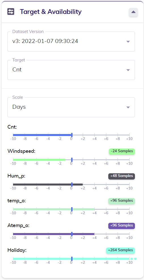
The card titled Target & Availability displays the availability of all variables in the dataset relative to that of the target. To view the overview of availabilities that's relevant to a specific use case, the user can select the desired version of the dataset and the intended target variable in this card. Following this, TIM Studio automatically determines an appropriate scale for looking at the availabilities (in the example image below, the scale is set to Days even though the dataset is sampled hourly); it is however possible to manually adjust this to a user's specific needs.
Below this scale, each variable present in the dataset is displayed together with a time axis indicating relative availabilities. The availability of the target variable (always 0) is indicated by the blue vertical mark. This way each variable's relative availability can easily be read: for example, the variable called Windspeed is available until one day before the end of the target variable, while the variable called Hum_p is available for two days after the end of the target variable. The exact relative availability of each variable is also displayed: this way it's easy to check that Windspeed's availability is indeed exactly 24 hours less than that of the target, and Holiday, which seemingly goes on into the future based on the time axis, is available for 264 samples or hours (11 days) past the end of the target variable Cnt.
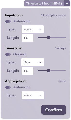
Data transformation
In the header section of the line chart card, a collapsed button can be found labeled Timescale. This button provides a summary of the sampling period (in the example below, 1 hour) and aggregation (in the example below, mean) of the data.
TIM makes it possible to adjust these settings, scaling, and aggregating the data according to the specific needs of the user's focus. An example use case can be seen in sales data, where sales may be measured hourly, but a daily forecast is desired. By scaling the data to a daily frequency and aggregating it by summation before starting the forecast, this objective can be achieved.
Timescaling can occur in set amounts of base units, with available base units being day, hour, minute, and second. Aggregation options include mean, sum, minimum, and maximum. The chosen aggregation method is applied to the target variable. By default, numerical variables are aggregated by mean, while boolean variables are aggregated by maximum.
Apart from timescale and aggregation, this menu also allows setting the imputation: i.e. are missing observations filled in and if so, how. It is possible to set the imputation type to Linear, LOCF (last observation carried forward) and None, the length can be set by specifying the maximal number of successive samples that should be imputed (this is not applicable for type None). By default, a linear imputation with a maximal length of 6 samples is applied.