build-model
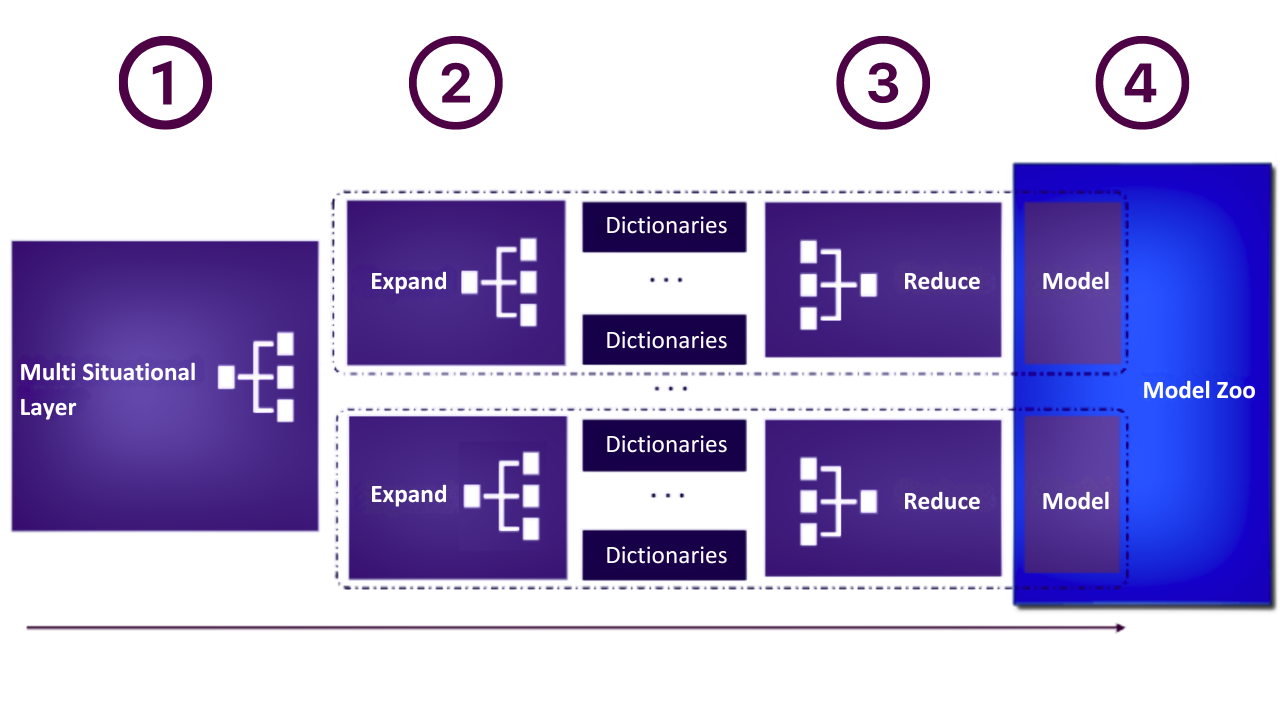
1. Multi Situational Layer
When building a Tangent model, the first step is passing the data and configuration through a Multi Situational Layer. This approach allows Tangent to create simple models for simple situations - like solar forecasting at night (where production is zero) - or sophisticated models when the situation requires complexity - like trading at the opening minute. Based on the Multi Situational Layer, which is automatically determined from the configuration and the data, Tangent will identify the various models that need to be build and stored within the model Zoo.
Example: Forecasting Energy Prices
Imagine forecasting energy prices on an hourly basis for the upcoming week. Tangent might identify different situational needs, such as:
Weekday Mornings
Weekday Afternoons
Weekday Evenings
Weekday Nights
Weekend Mornings
Weekend Afternoons
Weekend Evenings
Weekend Nights
In this scenario, Tangent would create eight distinct models, each tailored to these specific time periods and conditions. These models are then stored in the model zoo , allowing Tangent to apply the most appropriate model for each situation during forecasting.
Daily Cycle
A common situation that occurs is when daily cycles are detected in a dataset. The graph below displays the production of a typical solar farm over the course of one day. The objective of this use case is to forecast solar production. For example, predicting production at 3:00 AM is straightforward; a model that assumes production(t)=0 would likely be accurate since the sun does not shine at night. However, this same model would be inadequate for forecasting production at 12:00 PM, when solar activity is at its peak. This illustrates that the complexity of the model needs to vary depending on the specific time of day being forecasted.

one day solar production
Such datasets exhibit a "daily cycle," in contrast to "nondaily cycle" datasets. The difference between these two types of datasets can be easily observed in the images below.

daily cycle

non-daily cycle
Daily Cycle Detection
Tangent automatically detects daily cycles in a dataset if two key conditions are met:
Sampling Period: The dataset must have a sampling period between 10 minutes and 12 hours.
Below 10 Minutes: When the variance is too high, it is ineffective to build separate models for each time period.
Above 12 Hours: Insufficient data points within a day make it impossible to capture daily behaviors.
Data Span: The dataset should cover at least six months to ensure sufficient data for reliable pattern detection.
If these conditions are satisfied, Tangent performs an autocorrelation analysis:
Decreasing Autocorrelation: Indicates time-based patterns.
Regular Daily Spikes: Strongly suggest a daily cycle is present.
Handling Datasets with Daily Cycles
For datasets identified with a daily cycle, Tangent takes a specialized approach:
Time-Specific Models: TIM creates unique models for different times of the day, optimizing accuracy by accounting for distinct daily behaviors.
Backtesting and Rebuilding: The use of time-specific models means that backtesting and model rebuilding will differ from approaches used for non-daily cycle datasets.
The presence of a daily cycle is intrinsic to the dataset, so the entire Model Zoo will consist of either:
Time-Specific Models (for daily cycle data), or
Time-Generic Models (for nondaily cycle data).
Customization Options
TIM offers flexibility in how daily cycles are handled:
Force Daily Cycle Models: You can configure Tangent to use daily cycle models even if the cycle is not automatically detected, as long as the data meets the requirements.
Disable Daily Cycle Detection: Alternatively, you can prevent Tangent from detecting a daily cycle and use time-generic models instead.
These options give domain experts control, although Tangents' automatic detection generally provides the best results.
Importance of Time Zones
Correct time zone handling is critical when working with daily cycle models. Misalignment in time zones can lead to significant forecasting errors, as daily patterns may not correspond to the actual time of day. Ensure that time zone information is accurate to maintain model reliability.
2. N-Feature Expansions
Now, in the second phase of model building, Tangent will do a feature expansion for each separate model in the model Zoo. Here one creates numerous new features by transforming the original predictors in a meaningful way. Since these features have a one-to-one relationship with the target in the final model, they are inherently explainable. They clearly illustrate the direct relationship between each feature and the target variable.
Below is an overview of all possible transformations which are performed during the model building phase. Tangent finds relevant transformations automatically.
Identity
Transformation: PredictorName
Description: Uses the exact predictor value at the given timestamp without any time shifts.
Purpose: Filters predictors that can be used throughout the entire prediction horizon.
Application: Applied to numerical and boolean variables.
Time Offsets
Transformation: PredictorName(t - m)
Description: Reflects the time dependency of time-series data by introducing a delay or lag in the predictor values. The variable's timestamp is evaluated for the predictor
PredictorNamefrommsamples ago. This can include both past (e.g.,t-1for 12:00 tomorrow refers to 11:00 tomorrow) and, in some cases, future values (e.g.,t+1for 12:00 tomorrow refers to 13:00 tomorrow).Purpose: This is probably the most important dictionary. It is critical for capturing the temporal dynamics of the data, allowing the model to account for how past or future states influence the current prediction.
Application: Applied to numerical and boolean variables, excluding a delay of 0 as the Identity dictionary already covers this.
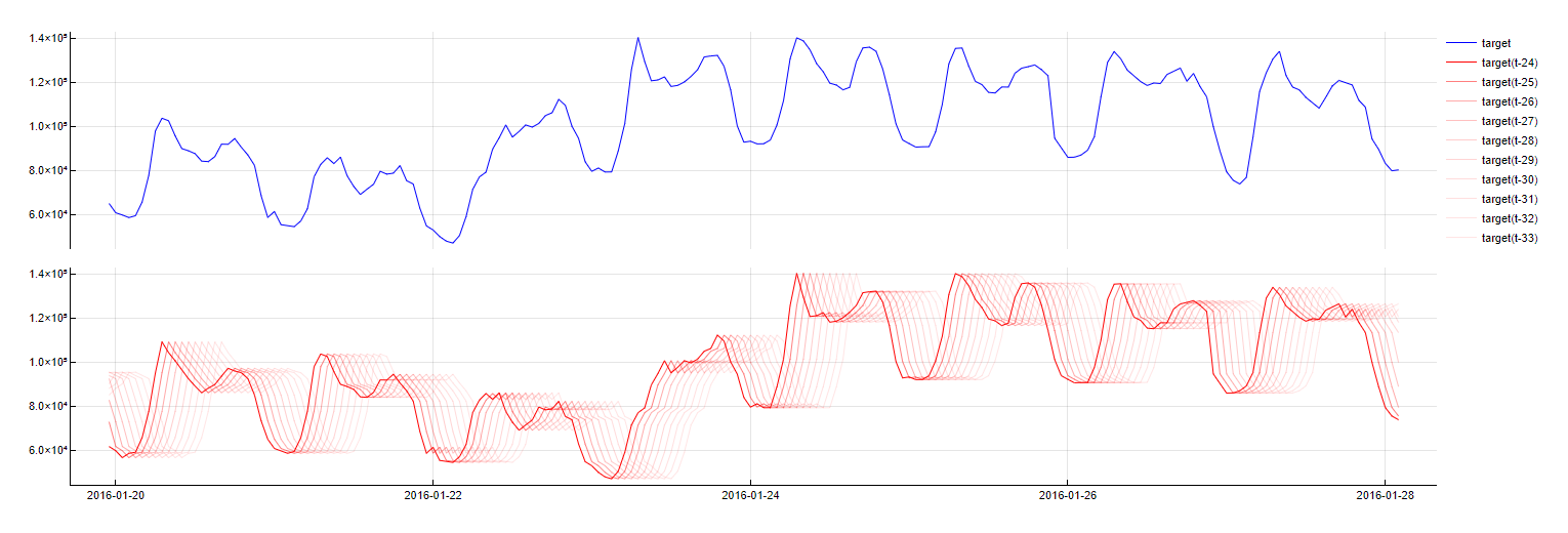
Time Offsets transformation
Weekday
Transformation: DoW(t - m) = NameOfDay
Description: Represents whether a timestamp belongs to a specific day of the week. For example, it can indicate whether the timestamp corresponds to a Monday, Tuesday, etc.
Purpose: Captures the weekly behavioral patterns that might influence the target variable, such as differences in sales volumes on weekdays versus weekends.
Application: Applied to boolean variables, with the possibility of including lagged values for enhanced model performance. It is not enabled by default but can be turned on as "Exact day of week".
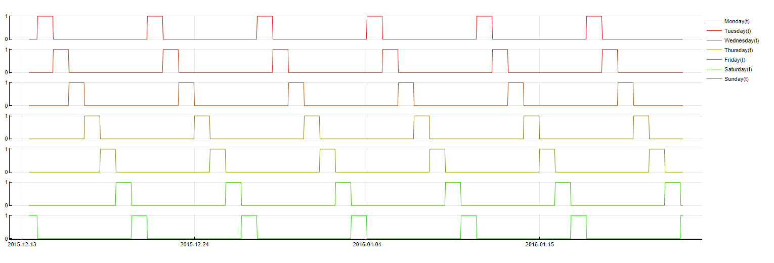
Weekday transformation
Weekrest
Transformation: DoW(t - m) ≤ NameOfDay
Description: Indicates whether a timestamp belongs to any of a specified group of days (e.g., Monday to Wednesday).
Purpose: More robust than single weekday indicators, this transformation captures broader patterns across multiple days, making it less prone to overfitting and reducing computation time.
Application: Applied by default in Tangent, especially useful for time series where specific day-of-week effects are too granular.

Weekrest transformation
Month
Transformation: Month ≤ NameOfMonth
Description: Tracks whether a timestamp falls within certain months of the year.
Purpose: Intended to capture seasonal patterns that recur annually. However, due to the limited number of distinct months, this transformation often does not significantly improve accuracy. To make it more stable we use the "rest" (see above) version and do not use time lags.
Application: Applied to boolean variables, often in a "rest" version without time lags to improve stability.

Month transformation
Public Holidays
Transformation: PublicHoliday(t - m), PublicHoliday(t + m)
Description: Indicates whether a timestamp corresponds to a public holiday or weekend, including the effects of days before and after holidays. Positive and negative time lags are used to model these effects.
Purpose: Captures the impact of non-working days, which can cause significant deviations in the target variable. By including weekends, the training set of non-working days is expanded. Days before, after or in between non-working days usually have specific behavior as well, e.g. bridge days. Therefore this dictionary generates negative and positive time-lags of the new variable.
Application: Applied to a single boolean variable designated as the
Holidaytype, which must be configured by the user.

Public Holiday transformation
Periodic Decomposition
Transformation: Sin(period, unit), Cos(period, unit)
Description: Decomposes the time series into sinusoidal components based on identified periodic cycles (e.g., daily, weekly).
Purpose: Humans tend to behave in cycles. Whether it is a daily cycle, a weekly cycle (such as represented by the weekdays dictionary) or something more uncommon, it often benefits performance to identify these cycles, their phases and their periods and incorporate corresponding variables in the models. Tangent focuses on common periods like 24, 12, 6, and 168 hours for 24-hour granularity.
Application: This transformation is often applied when periodic behavior is expected, enhancing model performance by adding relevant cyclical information.

Periodic Decomposition transformation
Fourier
Transformation: Fourier(period)
Description: Uses Fourier transformation to decompose the signal into sine and cosine waves, effectively modeling the entire time series as a combination of these periodic components.
Purpose: Useful for modeling time series that do not rely on time lags or have limited observations. The transformation aggregates all signals to approximate the target variable more accurately.
Application: While powerful, this transformation can result in a large number of coefficients, making it complex but effective for specific types of time series data. As there are usually too many components, we only display the period tag in the feature decomposition.

Fourier transformation
Piecewise Linearity
Transformation: max(0, knot - PredictorName(t - m)), max(0, PredictorName(t - m) - knot)
Description: Splits a variable into different regimes based on specified "knots," allowing different linear relationships in each segment. Tangent identifies relevant knots and time lags to optimize the model.
Purpose: Addresses non-linear relationships between predictors and the target variable, improving the model's ability to fit data that exhibit varying, irregular behaviors across different ranges.
Application: Applied to numerical variables, providing a flexible approach to handle non-linearity in the data.
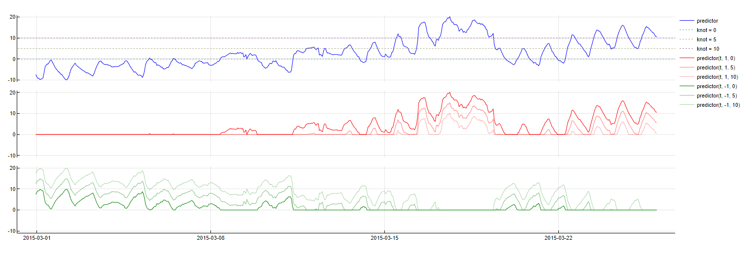
Piecewise Linear transformation
Simple Moving Average
Transformation: SMA_PredictorName(t - m, w = window)
Description: Computes the simple moving average of a predictor over a specified window, up to
msamples before the current timestamp.Purpose: To smooth out short-term fluctuations and highlight longer-term trends, compensating for higher scale changes in the predictor values.
Application: Applied to numerical variables, with Tangent finding the optimal window length to balance responsiveness and smoothness.
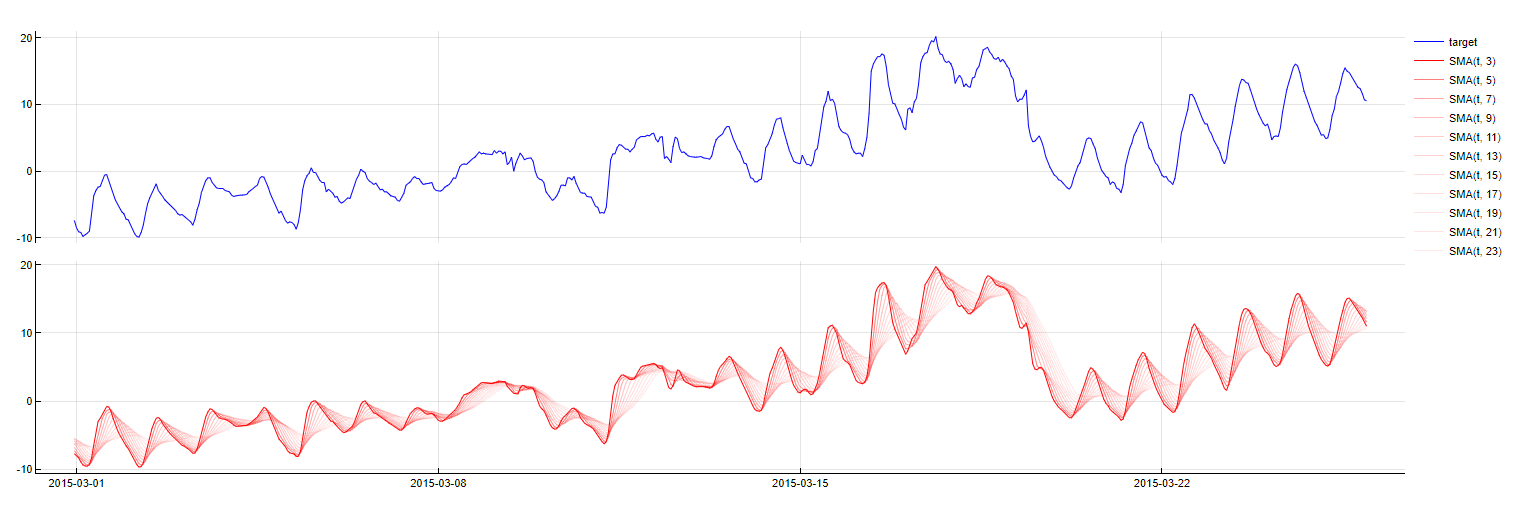
SMA transformation
Exponential Moving Average
Transformation: EMA_PredictorName(t - m, w = window)
Description: Similar to SMA but gives more weight to recent observations, creating a weighted moving average. Tangent optimizes the weight parameter to enhance model accuracy.
Purpose: To capture recent trends more effectively, with more emphasis on the most recent data points.
Application: Typically applied to the target variable, with SMA used as a fallback when calibration data is insufficient. This transformation can be helpful to capture peaks as it might overfit to the more recent patterns.
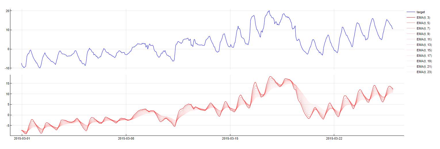
EMA transformation
Trend
Transformation: Trend(step)
Description: Represents the trend over specified time steps (e.g., hourly, daily, monthly), converting the timestamp into the number of steps since a reference date (time of forecasting).
Purpose: To amplify trend effects, especially when time lags of the target cannot be used. This transformation can help in identifying and emphasizing long-term trends.
Application: Applied to temporal data, providing a straightforward way to include trend information in the model.

Trend transformation
One-Hot Encoding
Transformation: PredictorName(t - m) = category
Description: Converts categorical variables into binary columns, with each column representing a unique category. If a data point belongs to a particular category, the corresponding column is set to 1, and all others to 0.
Purpose: Enables the inclusion of categorical variables in the model-building process, facilitating the handling of non-numeric data.
Application: Applied when categorical variables are present. It avoids transformation for predictors with more than 20 categories due to the potential explosion in the number of predictors.
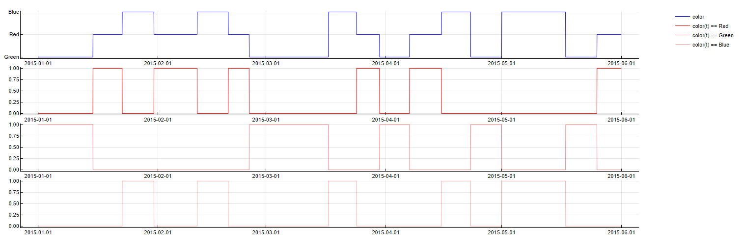
One-Hot Encoding transformation
Polynomial
Transformation: transformation1 x transformation2
Description: Models interactions between different predictors by taking element-wise products of two vectors, capturing second-degree interactions between variables.
Purpose: To capture complex interactions that may exist between different predictors, enhancing the model's ability to explain variations in the target variable.
Application: This transformation is applied last, allowing for the combination of features from all previous transformations to form more complex models.
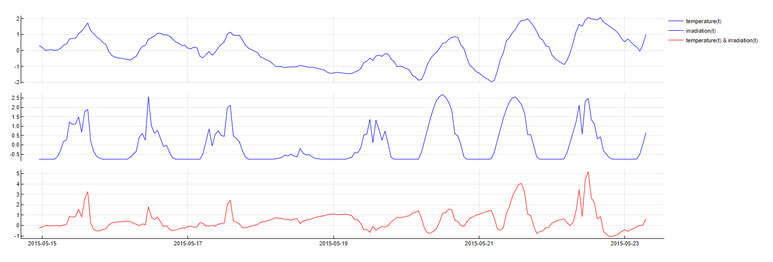
Polynomial transformation
Intercept
Transformation: Intercept
Description: Includes a constant value in the model, representing the mean of the target variable.
Purpose: To improve model performance by accounting for the baseline level of the target variable, ensuring that the model can adjust for the average value of the target.
Application: A simple yet effective transformation, typically included in most regression models to capture the mean level of the target variable.

Intercept transformation
3. N-Feature Reductions
The third stage of Tangent's model-building process involves feature reduction. In the previous stage, a large number of new features are generated. However, retaining all of these features in the final model is not optimal, as many may be correlated, leading to overfitting. Overfitting occurs when a model becomes too complex, capturing noise instead of the true underlying patterns, which makes the model unstable. To prevent this, only the most important subset of features is retained, reducing high correlation and improving the model's stability.
Feature reduction is a well-researched area, with commonly known techniques like LASSO, PCA, and forward regression. Tangent employs a similar approach that relies on a geometrical perspective and incorporates a tweaked Bayesian Information Criterion to select the optimal subset of features.
This process is closely tied to the bias-variance trade-off:
Too Simple (High Bias): If Tangent retains too few features, the model may become too simple, resulting in high bias and underfitting. This means the model fails to capture important trends in the data, leading to poor predictions.
Too Complex (High Variance): On the other hand, if too many features are retained, the model may become overly complex, leading to high variance and overfitting. This means the model performs well on training data but poorly on new, unseen data, as it has learned to capture noise rather than the true signal.
The goal of Tangent's feature reduction process is to strike the right balance between bias and variance. By carefully selecting the most relevant features, Tangent minimizes both bias and variance, resulting in a stable and accurate model that generalizes well to new data.
Bias variance trade-off (Geman, S., & Geman, D. (1992). IEEE Trans. PAMI, 6(6), 721–741.)
4. Model Zoo
The Model Zoo is a dynamic repository where all the individual models created during Tangent’s multi-situational analysis are stored and managed. It plays a crucial role in ensuring that the right model is applied to the right situation, optimizing both accuracy and efficiency.
By leveraging the Model Zoo, Tangent ensures that the most appropriate model is always used, delivering accurate and reliable forecasts tailored to the specific needs of each situation, such as the time of forecasting, the forecasting horizon, and data availability.
Consider a one-day-ahead forecast of the Belgian grid load at an hourly sampling rate. In this scenario, the Model Zoo, contains 24 individual models—one for each hour of the day. Since grid load is closely tied to human behavior and thus cyclical variations, Tangent automatically generates a distinct model for each hour, significantly improving the forecasting accuracy.
In the example provided, the model for 14:00 is shown. As seen in the second plot, each model is composed of a linear combination of features (or terms) and coefficients. These features are the outcome of the expansion and reduction phase described earlier. The normalized coefficients, much like in any regression, indicate the impact of each feature on the target variable, which in this case is the grid load.
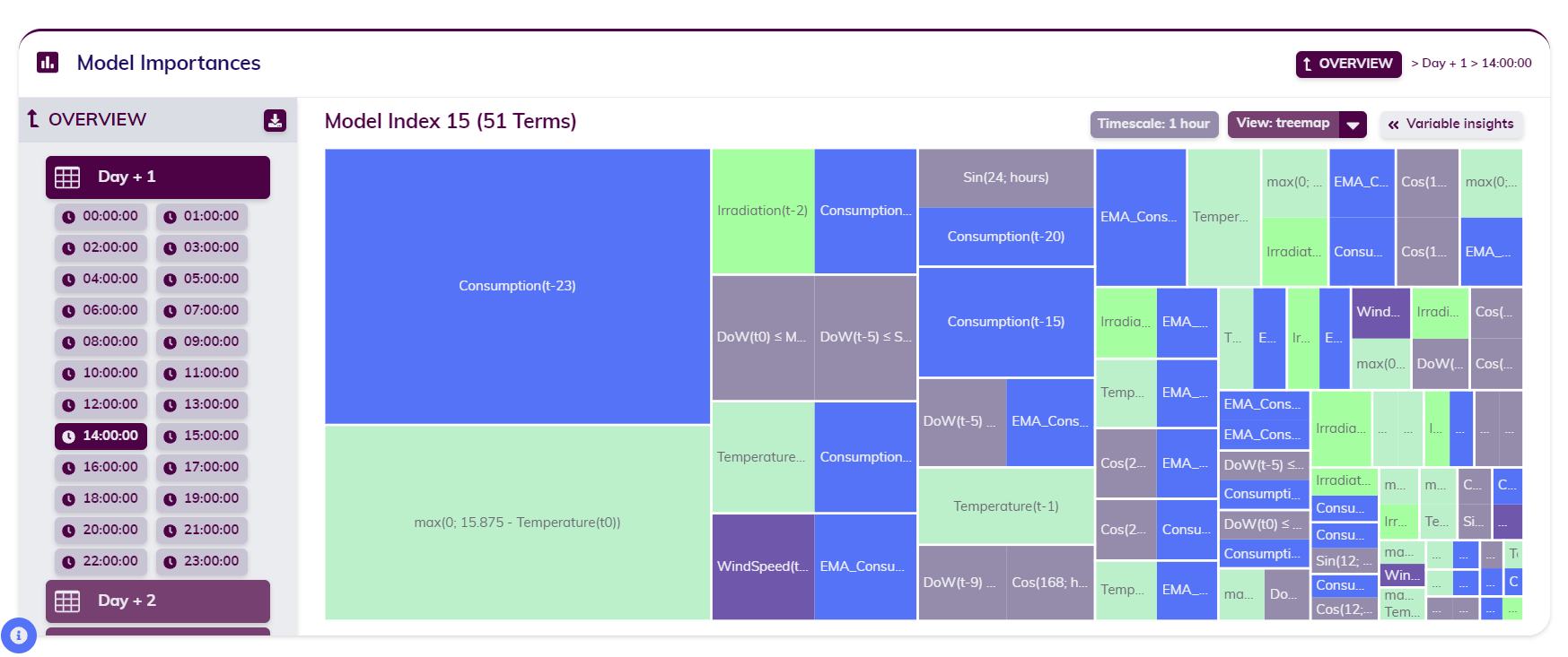
single model in the Model Zoo - treemap view
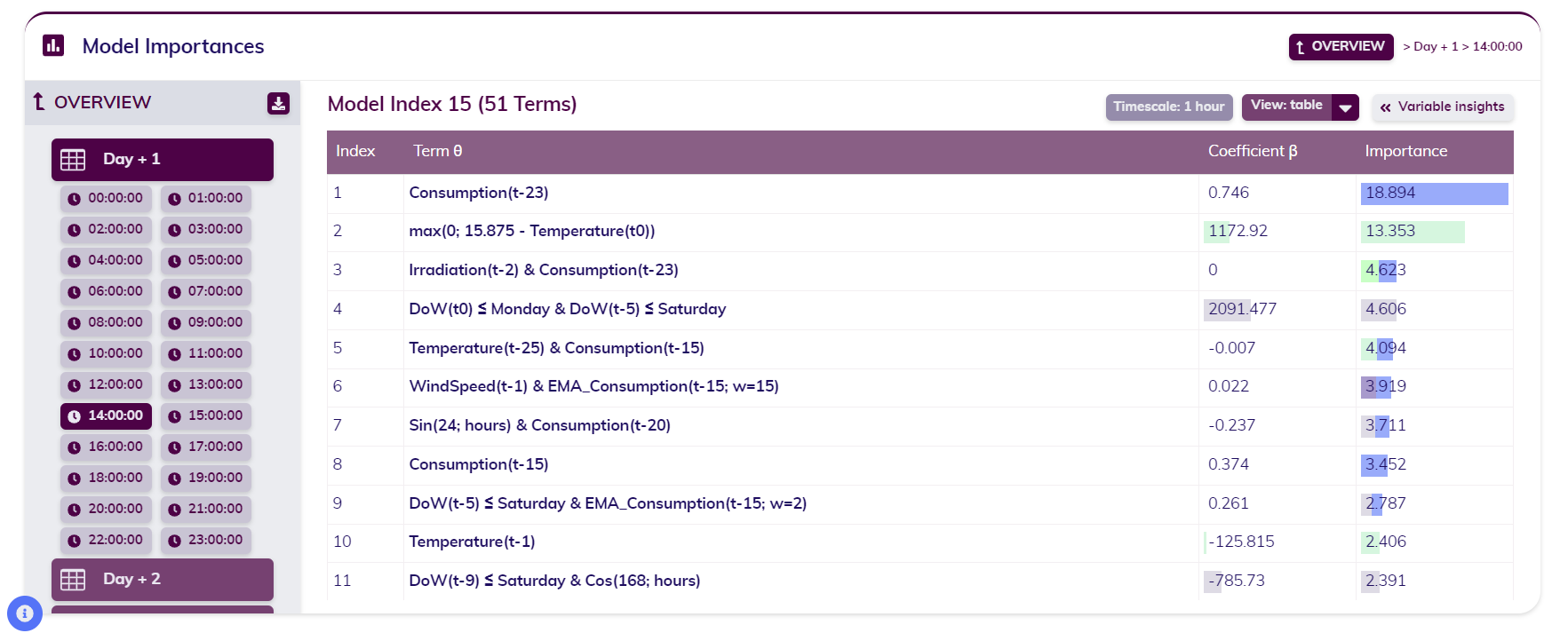
single model in the Model Zoo - table view
