What-if analysis
Introduction
What-if analysis is a powerful tool that allows users to explore hypothetical scenarios of 'what if' by modifying input variables and observing the resulting changes in model outputs. This type of analysis is essential for understanding the impact of specific variables on Key Performance Indicators (KPIs) or anomaly detection outcomes. Whether applied to forecasting or anomaly detection, what-if analysis helps users make informed decisions, optimize processes, and identify potential risks.
How It Works
What-if analysis can be applied in both forecasting and anomaly detection contexts:
Forecasting: Users can simulate different scenarios by altering predictor variables to see how these changes impact future predictions. This helps in assessing the sensitivity of forecasts to certain inputs and identifying key drivers of forecasted outcomes.
Anomaly Detection: In anomaly detection, what-if analysis allows users to modify inputs to understand their effect on the detection of anomalies. This can reveal which variables contribute to abnormal behavior and under what conditions the system would consider these behaviors as normal.
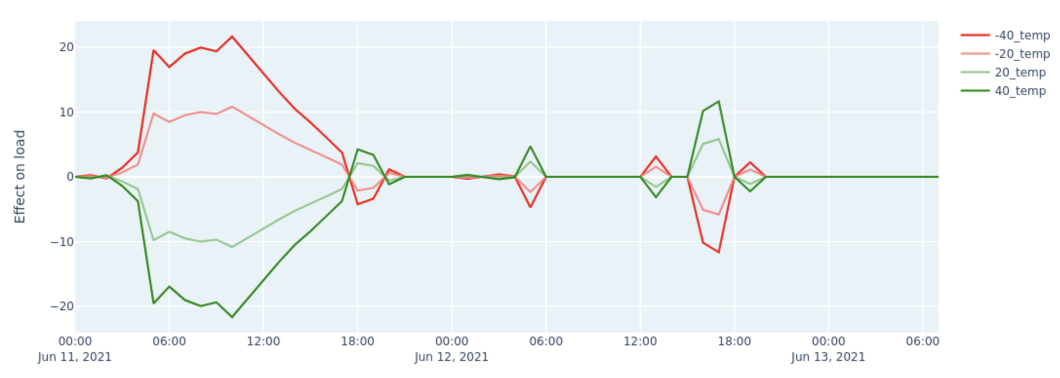
what-if global: effect of temperature on grid load
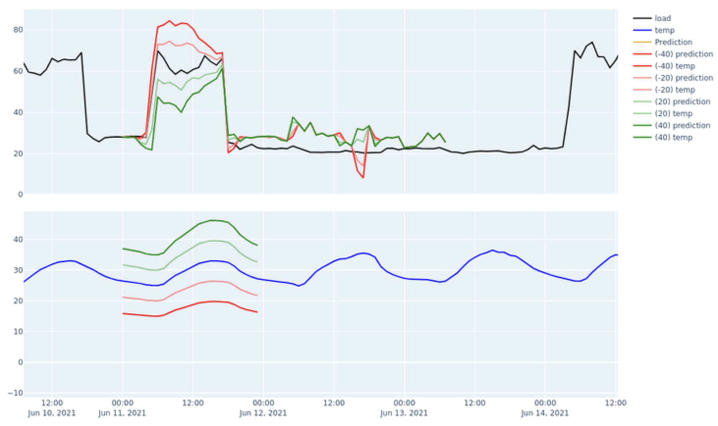
what-if local: effect of temperature on grid load
Example Scenario: Grid Load Analysis
In this scenario, we are focusing on forecasting the grid load in the European market. The model is trained using historical data, where key predictors include wind speed, temperature, and humidity. These factors are known to influence energy consumption patterns significantly. The objective is to understand how variations in these predictors, specifically temperature, impact grid load during different times of the day.
What-If Configuration
To explore the impact of temperature variations on grid load, the following what-if analysis configuration is applied:
Temperature Adjustments:
Top Graph Analysis:
The black line represents the actual grid load.
The blue line indicates the unadjusted temperature.
Colored lines represent different temperature adjustments and their impact on load predictions:
Red Lines: Correspond to -40% (darker red) and -20% (lighter red) temperature scenarios.
Green Lines: Correspond to +20% (lighter green) and +40% (darker green) temperature scenarios.
Bottom Graph Analysis:
The blue line shows the actual temperature over time.
The red and green lines reflect temperature adjustments corresponding to the scenarios analyzed in the top graph.
Time of Day Impact:
The analysis is segmented across different times, from early morning through to late evening, to understand the dynamic response of grid load to temperature changes.
The analysis reveals the following insights:
Morning Impact:
Lower temperatures lead to a sharp increase in grid load due to higher heating demands, which is consistent with typical energy consumption patterns during colder mornings.
Midday Neutrality:
The minimal effect observed during midday suggests that temperature fluctuations do not significantly alter grid load, possibly due to the offsetting effects of reduced heating and increased cooling or stable industrial energy use.
Evening Complexity:
The varying effects in the evening indicate that temperature changes influence energy consumption differently depending on specific evening activities, regional behaviors, and potential cooling demands, especially in the case of higher temperatures.
Conclusion
The graph highlights how temperature adjustments impact grid load throughout the day. The most significant changes are observed during the morning and evening periods, where temperature reductions cause an increase in grid load, while temperature increases generally lead to a decrease. The midday period shows minimal sensitivity to temperature changes. Understanding these patterns can help grid operators anticipate demand changes and adjust supply strategies accordingly.