Experiments
![]()
An experiment is the working point in the TIM platform, where users will find the core of the analytics. Each experiment is focused on a single type of analytics:
- Forecasting experiment - used for forecasting and classification.
- Anomaly detection experiment - used for KPI-driven, system-driven, and outlier detection.
- Drift detection experiment - designed for detecting drift, although it is not currently visible in the TIM Studio.
The experiments overview
As experiments can be found a single level deep inside use cases, the experiments overview page is the same page as the use case detail page. More information on the experiments overview page can be found in the section on the use case in detail.
The experiment in detail
The detail view of an expriment exposes different view modes. Using the view mode menu allows a user to switch between those view modes.

Detail view mode
In an experiment's detail page (jobs overview page), all of the information regarding the experiment can be found. That includes the name, description and type (forecasting or anomaly detection), as well as the dataset and dataset version it revolves around and information on all of the iterations (jobs) it contains.
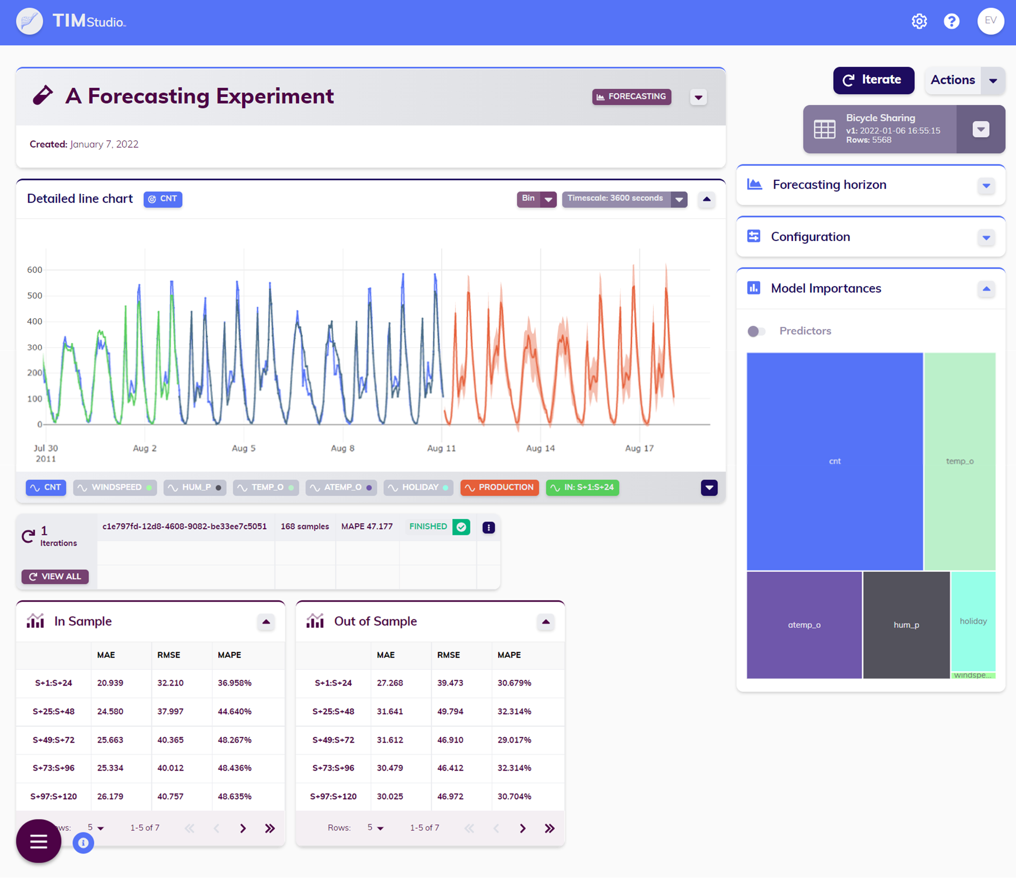
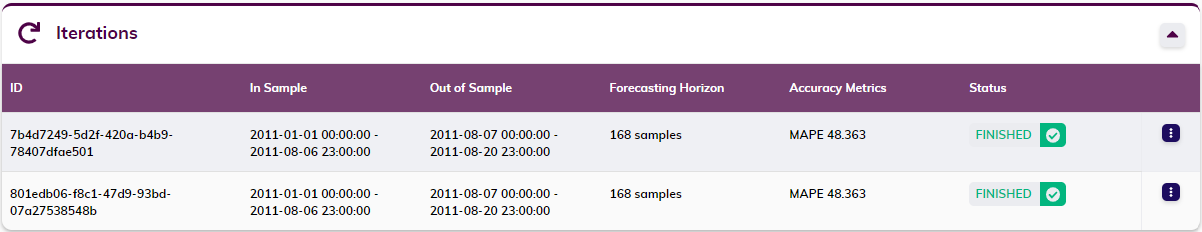
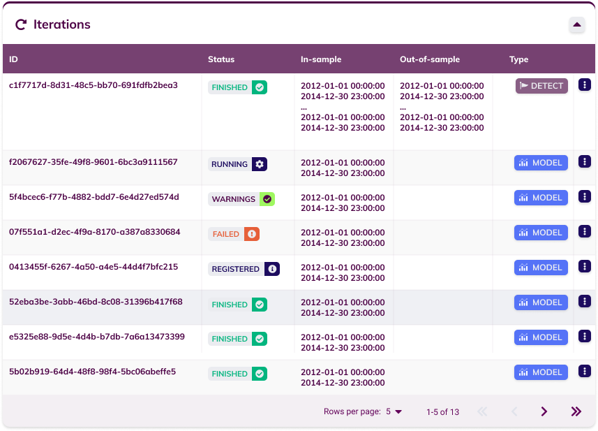
The Iterations table provides an overview of all the jobs that are contained in the experiment. For each job (each row in the table), important configuration settings (in-sample and out-of-sample ranges, the forecasting horizon for forecasting jobs, and the job type for anomaly detection jobs) are displayed, as well as the job's status. If the job has been executed successfully (status Finished or Finished With Warning) its aggregated MAPE (Mean Average Percentage Error) is shown too. Clicking a job that has been executed successfully opens up that job's results.
That is not all; more on the specifics of this page follows below.
From this page, a user can edit or delete the experiment. From the iterations table, a user can delete a job/an iteration.
Editing: Editing an experiment allows the user to update its name and description.
Deleting: Be careful with deleting an experiment: deleting an experiment will also permanently delete any data contained in this experiment, including the ML jobs.
Deleting a job/an iteration: Deleting a job/an iteration will delete its
Opening an experiment: a clean slate
Within an experiment, users get to explore the data, again, and can browse through configuration options. An overview of the configuration options can be found in the dedicated sections on the configuration for forecasting and the configuration for anomaly detection. The user can also inspect the variables' availabilities relative to the target or KPI similar to how this can be done on the data availability component on a dataset's detail page
Once the desired settings are selected, an ML request can be triggered and TIM Studio will show how the calculation progresses. This request involves the creation of a new job, which will be added to the Iterations table.
Dataset overview and configuration
The component visualizing the dataset version used in the experiment, along with some of its details, can be expanded to a larger card. This larger card displays more information and exposes additional configuration options related to the data, such as
- metadata describing the currently selected version,
- the selected dataset version,
- the selected target or KPI,
- available variable related configuration,
- available range related configuration and
- the dataset's alignment or variable availabilities.
There is a reset button in the card's header ![]() that serves to reset all data configuration settings to their default value.
that serves to reset all data configuration settings to their default value.
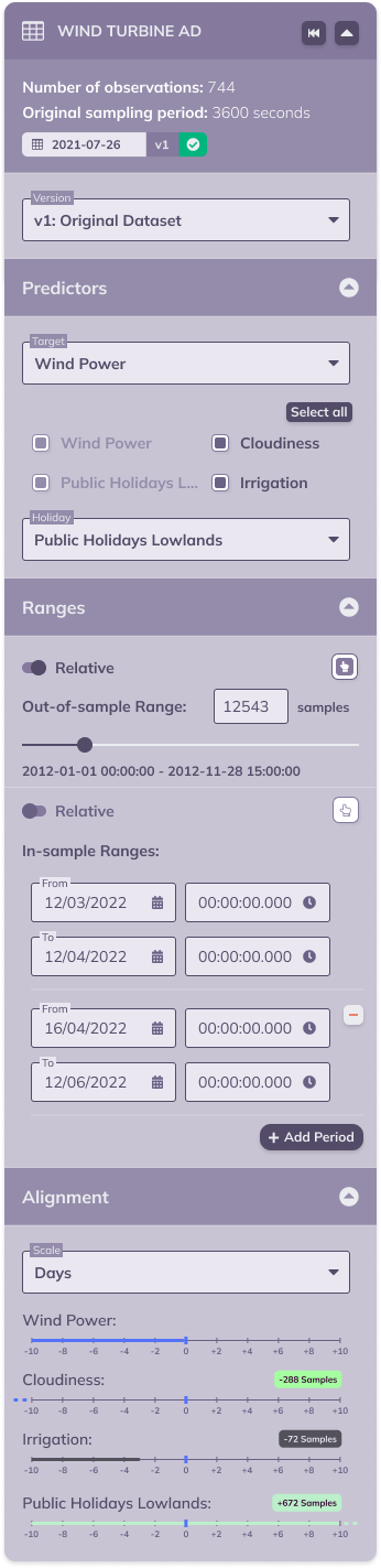
The image below shows a version of the expanded dataset card with maximal content and expanded subsections; when a user comes across this card in TIM Studio it will either be in this fashion or with just the available subset of configuration options.
The dataset version
The selected dataset version and some of its metadata is already displayed in the collapsed version of the dataset overview. In the expanded version however, it is also possible to change the selected version, and other displayed information will change accordingly. The version that is selected when registering a job will be used for that job.
The target or KPI
To facilitate the user in keeping an overview of the experiment, the selected target (TIM Forecast) or KPI (TIM Detect) is displayed in the header of the line chart card. In the expanded dataset card however, it is also possible to change the selected target or KPI, and the other displayed information will change accordingly. The target or KPI that is selected when registering a job will be used for that job.
Predictors or influencers
Where available, the dataset card shows a configuration section for settings related to predictors (TIM Forecast) or influencers (TIM Detect). In this section, it is possible to set the target variable (TIM Forecast) or KPI variable (TIM Detect's kpi-driven approach), to select the variables that should be included for model building, and to set the holiday variable.
Ranges
Where available, the dataset card shows a configuration section for settings related to ranges. This can include in-sample ranges, out-of-sample ranges or both. Both types of ranges can be set interactively through selection in the line chart by selecting the appropriate icon next to the setting: ![]() . Both settings are available in an absolute fashion - by specifying the start and end timestamp of each (sub)range - and in a relative fashion - by specifying the amount of samples counting from the end of the dataset version. The switch accompanying the setting allows switching between both options.
. Both settings are available in an absolute fashion - by specifying the start and end timestamp of each (sub)range - and in a relative fashion - by specifying the amount of samples counting from the end of the dataset version. The switch accompanying the setting allows switching between both options.
Dataset alignment or variable availabilities
The variable availabilities display the availabilities of all variables in the selected dataset version relative to that of the selected target or KPI. TIM Studio automatically determines an appropriate scale for looking at the availabilities (in the example image above, the scale is set to Days even though the dataset is sampled hourly); it is however possible to manually adjust this to a user's specific needs.
Below this scale, each variable present in the dataset is displayed together with a time axis indicating relative availabilities. The availability of the target or KPI variable (always 0) is indicated by the blue vertical mark. This way each variable's relative availability can easily be read: for example, the variable called Irrigation is available until three days before the end of the target or KPI variable. The exact relative availability of each variable is also displayed: this way it's easy to check that Irrigation's availability is indeed exactly 72 samples or hours less than that of the target or KPI, Cloudiness, which seemingly goes into the past based on the time axis, is available until 288 samples or hours (12 days) before the end of the target (or KPI) variable and Public Holidays Lowlands, which seemingly goes on into the future based on the time axis, is available for 672 samples or hours (28 days or 4 weeks) past the end of the target (or KPI) variable Wind Power.
Data transformation
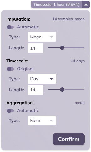
In the header section of the line chart card, a collapsed button can be found labeled Timescale. This button provides a summary of the sampling period (in the example below, or 1 hour) and aggregation (in the example below, mean) of the data.
TIM makes it possible to adjust these settings, and scale and aggregate the data to the specific needs of the challenge a user is focusing on. A potential use case here can be found in sales data, where sales may be measured hourly, but a daily forecast is desired; scaling the data to a daily frequency while aggregation by summation before starting the forecast would achieve this.
Timescaling can happen on set amounts of base units, with available base units being day, hour, minute and second. Aggregation is available by mean, sum, minimum and maximum. The aggregation that is set relates to the target variable. By default, numerical variables are aggregated by mean and boolean variables are aggregated by maximum.
Apart from timescale and aggregation, this menu also allows setting the imputation: i.e. are missing observations filled in and if so, how. It is possible to set the imputation type to Linear, LOCF (last observation carried forward) and None, the length can be set by specifying the maximal number of successive samples that should be imputed (this is not applicable for type None). By default, a linear imputation with a maximal length of 6 samples is applied.
Any imputation, timescale and aggregation that is configured, will also take effect on model building and model application, and thus on the results of a forecasting or anomaly detection job.
The results of a job
After the model has been built and applied (or when browsing to a job that has already been executed), it’s time to examine the results. Users can get insights into the models that were used and review the performance.
Find out more about a job's results in the sections about forecasting experiments and anomaly detection experiments.
The Model Zoo
The job's result include its Model Zoo, which is visualized on the experiment page. More information on the way the Model Zoo is visualized can be found in the documentation section dedicated to the Model Zoo in TIM Studio.
The job's configuration
Users can adjust the configuration where needed by iterating over the job. Therefore, it is relevant to be able to review a particular job's configuration if it has already been successfully executed. The same configuration cards that are used to set a job's configuration when creating a job can be used to review an existing job's configuration. This time the settings will be disabled from changes, to avoid confusion as to what a user is looking at (the configuration used for an existing job versus the configuration to be used for a new job).
For an overview of the configuration options as they are presented to the user in TIM Studio, take a look at the sections about forecasting experiments and anomaly detection experiments.
The process of iterating
After the results of a job have been examined, a user may want to continue experimenting and iterate over that job to find ways to improve the results. The Iterate button allows the user to do just that. When clicked, it will bring the user back to the clean slate state of the experiment, with one exception: the configuration will remain as it was in the previously looked at job. Therefore, the user does not have to restart from the default configuration when setting the configuration; they can adjust the previous configuration as desired.
Operations view mode
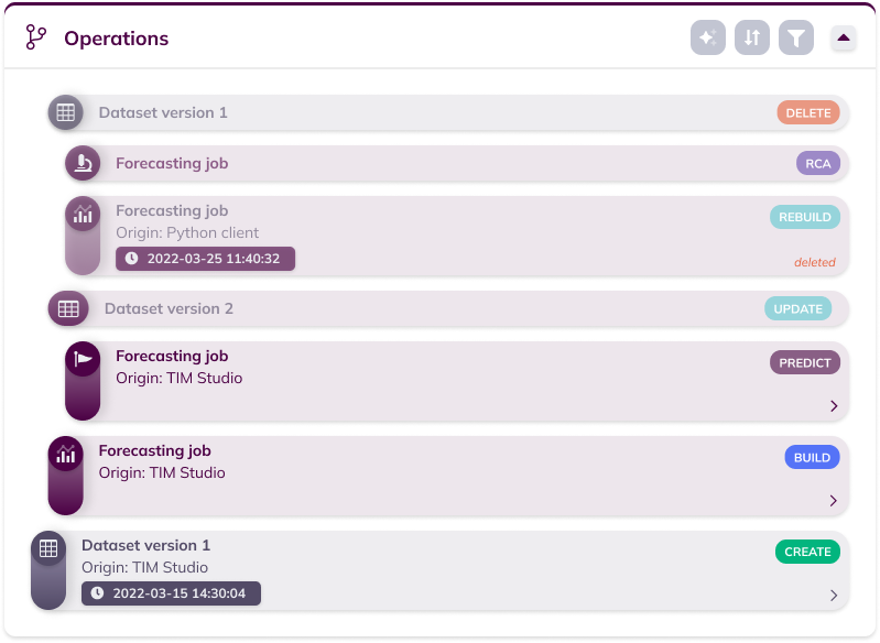
The Operations view mode contains an overview of the history of the experiment, in other words all operations that happened related to the experiment.
These operations include any jobs created in this experiment, as well as any dataset uploads and updates used for these jobs. Each operation is visualized in its own component. If the related entity (dataset version or job) has been deleted since, the operation has an opacity to reflect this. If the related entity still exists, the arrow at the bottom right of the operation allows navigating to it. The icon at the left of the operation shows the operation subtype (dataset; job: model building, model application, RCA) and allows to expand and collapse the operation to see more (or less) of its metadata. This metadata includes the origin indicating the interface from which the operation was performed and the datetime of the operation. At the top right of each operation, the operation's action type (dataset: create, update, delete; job: build, rebuild, predict, detect, RCA) is displayed.
The operations card also contains a set of action buttons that can be used to manipulate the way in which the operations are shown. The sections below explain the possibilities of each of these actions.
Sorting

The sorting menu enables setting the order in which the operations are shown. By default, the most recent operations are shown first (i.e. reverse chronological order). It is possible to revert this and show the olders operations first by clicking the arrow button next to "Chronological".
Filters

The filter menu enables defining which operations to include in the list and which operations to exclude from the list. By default, all operations are included. The "Existing" and "Deleted" options filter on the state of the related entity (dataset version or job).
Hover relations

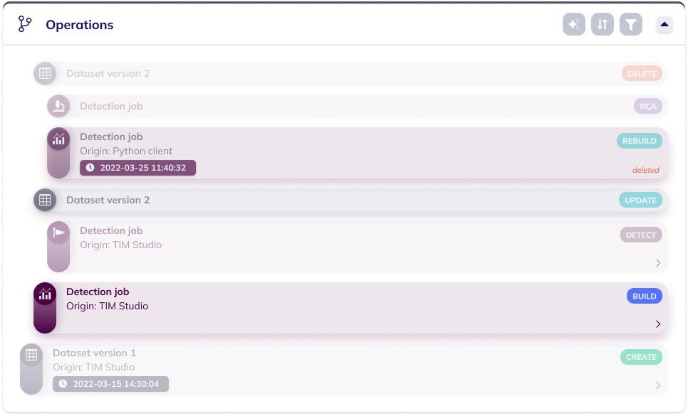
The hover relations menu enables to easily visualize relations between operations that are of interests. The "Parents" options allows for showing an operation's parents (the parent (dataset)/used (job) dataset version and, if applicable (job), the parent job), while the "Children" operation allows for showing an operation's children (the descendant dataset version (dataset) or jobs (job)).
When one or both of these options are selected, hovering an operation will bring forward that operation's relation(s) of choice, as shown in the image below.
Production evaluation view mode
The production evaluation view mode visualizes the results of a sequence of jobs. Currently, this view mode is only available for forecasting experiments.